In the last two posts, we’ve looked at the big picture outputs of the xG model for players and teams. Now, let’s zoom in on the model itself to try and understand it better. How is it making its decisions? Which variables provide the most important information and in what way do those variables affect the outcome?

This is important for several reasons. For the model builder, it helps check assumptions and suggest improvements for further development. For example, if screens are extremely important in some cases but not others then we would want to spend time in a future model building additional features that get more details about the screen like the distance of the screener from the shooter. But if the model says that shots from further away from the net are always better than we can pretty safely say that something is broken and we need to check everything for bugs.

For people using the model, understanding the features is essential to understanding player evaluation and tactical decisions. The more important features help explain what players may be doing to drive particularly impressive results. And identifying valuable shot types can lead to tactical changes that create more of those chances.

More generally, it’s just important to understand how each piece of information affects the results. Even things that we think are straightforward may prove counterintuitive. For example, I had been assuming that having a screen on a shot would naturally lead to better results. However, David Yu of SportLogiq pointed out that I had been thinking about it too simplistically: since screens indicate people between the shooter and the goalie, they may also be correlated with defensive pressure on the shooter, which could decrease shooting percentage. At the very least, this was a hypothesis deserving of investigation.

We already have a rough sense of variable importance. In my first post on this model, I showed this chart:

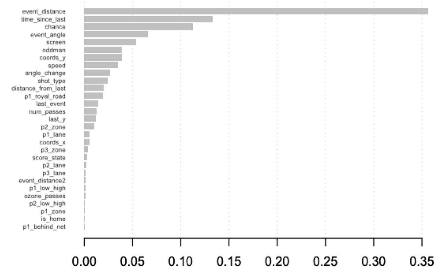
This chart shows the “Gain” of each variable in the XGBoost model; essentially, it shows how much better the model gets when it starts using that variable to help it make decisions. That’s an oversimplification, but it is enough for us to get a general sense of which variables matter. As I said at the time:

Unsurprisingly, the traditional features available in play-by-play data remain extremely important; the single most important feature by a wide margin is how close the shot is to the net. Other pbp features like the time since the last event and the angle of the shot also remain very important. We can then see where the pre-shot data becomes useful. The model gets valuable information out of the flag that indicates whether the shot comes from the scoring chance area, whether the shot was screened, and whether it involved an oddman rush.

But we can do more to dig deeper into specific variables. For example, the distance and angle makes it clear that the location of the shot matters, but in what ways? We can answer that by graphing the mean xG from every location:

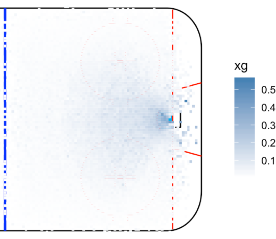
Here we validate the traditional “home plate” area; the most dangerous area of the ice is directly in front of the net, followed by the inner slot between the face-off dots.

Other features are a bit more complex, so we’ll dig into each of them in turn. First, we’ll look at features of the shot itself: screens, scoring chances, and oddman rushes. After that, we’ll look at details of the pass final pass before the shot occurred.

Shot Types

Shooting from a scoring chance area, getting a screen, and shooting off an oddman rush are all important features that we intuitively expect would increase scoring. However, we don’t know the scale of the impact or how different types of oddman rushes compare. Let’s start by looking at the median xG for shots of each type in our dataset:

These results match our intuition: shots with a screen have double the shooting percentage as shots without, and scoring chances are more than triple as likely to go in. In addition, oddman rushes are extremely good scoring chances; the success of 3-on-2 rushes is surprising, but could be the result of a small sample; the rest of the values generally make sense.

However, this does not really isolate the value of these features. These features could very easily be correlated with other important variables that also play into these differences. For example, maybe shots with a road road pass are extremely likely to come from a scoring chance area. In that case, scoring chances would do much better than not, but the magnitude of difference above is also including the royal road passes that are more likely to occur on the scoring chance shots.

To adjust for this, we’ll turn to some more advanced techniques. First, we can look at the Shapley values of each variable. Shapley values come from game theory and are used to distribute credit fairly between multiple contributors. In this case, we can look at each shot and see how much credit for the miss or goal should be attributed to each variable in the model:

In these charts, each dot is a shot. The x-axis divides them up into shots that did or did not have that particular feature, and the y-axis shows their Shapley value. That is, we can see how much that feature changed the prediction of that shot from just being the average prediction of the data.

In this case, we can see that the Shapley value matters quite a bit when there is a scoring chance or a screen. Also, notice how the spread of points is much bigger for screened shots than non-screened shots or scoring chances. This means that there is likely a lot of interaction between screens and other variables; the results of screened shots can vary quite widely depending on other data about the shot.

Finally, we can use one other technique I particularly like: duplicating datasets. We can make copies of our dataset and then change the variable in question so that we have two datasets: one where the variable is always true and one where it is always false. We can then get predicted xG values of every shot in both datasets and see how much the prediction changes. Here is the distribution of those differences for scoring chances and screens:

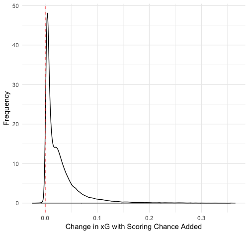
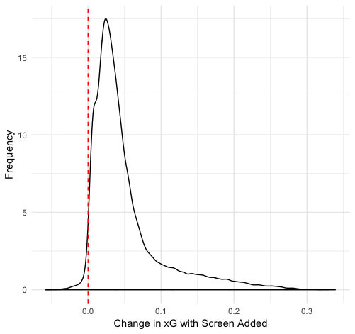
We can see that the affect of a scoring chance or screen changes from shot to shot, but generally is a small increase. There’s plenty of variation: on some shots they increase the xG by 0.3, and in a few cases they even decrease xG. But typically there is a 1-2% increase in shooting percentage if there is a scoring chance and a 2-3% increase if there is a screen.

Why does a screen add more value than a scoring chance area despite the original data differences suggesting the opposite? I suspect it is the result of the relationship between these variables and others in the data. Scoring chances are just combinations of x and y coordinates, which are also included as features. Even when the chance area is changed to false, the model still has that location information encoded in the value.

Pass Types

Now let’s look at the types of passes that can occur before a shot. For simplicity, we’re going to focus on the pass immediately before the shot and ignore any others that may have happened earlier. First, where should the shot come from to be as dangerous as possible? Let’s look at the real data we have on hand:

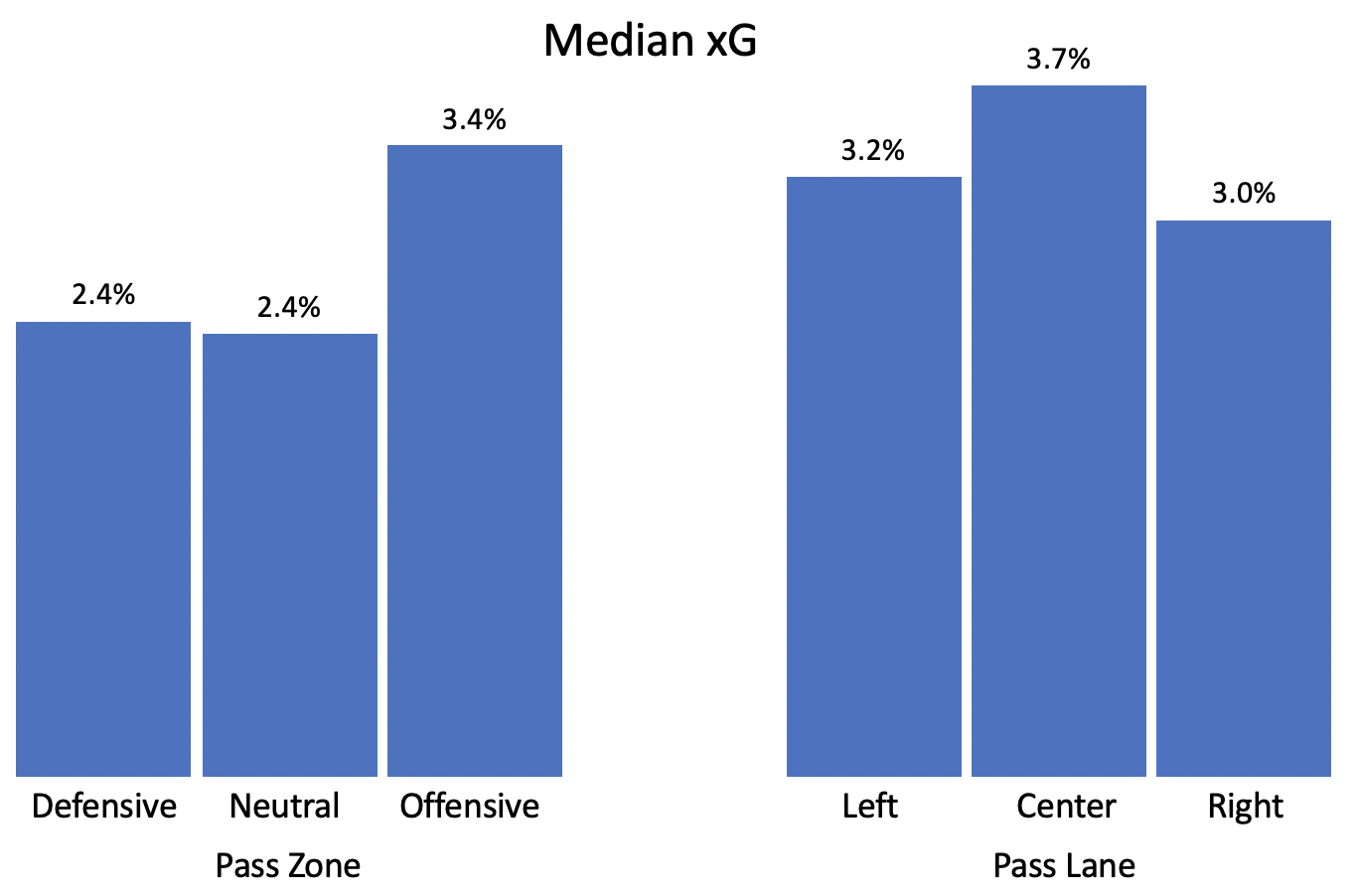
This all checks out. A pass is most dangerous if it comes from the center lane of the offensive zone. Other than that, the zone and lane do not matter very much. This isn’t surprising to anyone who has watched hockey: these passes require the defense to react and the center lane provides the most options. The more advanced methods back this up as well, so I won’t spend any more time on it.

What about the type of pass? We track a few different kinds, and they are largely coachable. If particular ones are better than others, the team can develop systems to encourage that sort of play. Similar to what Ryan Stimson has previously done, let’s look at the data:

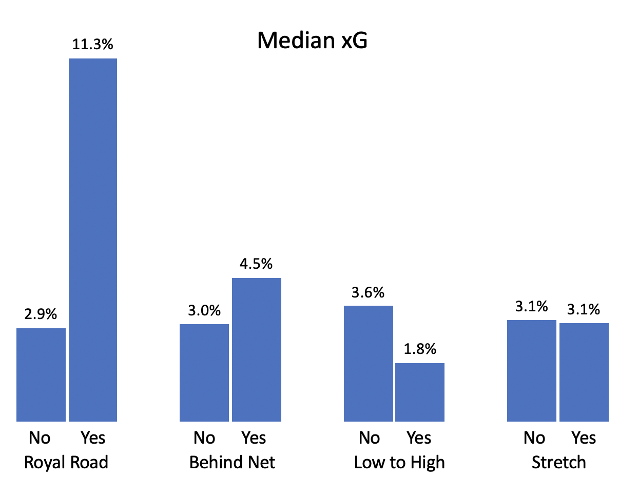
The one that sticks out here is royal road passes: shots are much more likely to score if they come after a pass that moves across the ice in front of the goalie. Passes from behind the new do a bit better while stretch passes are no better or worse than other passes. Passes from low to high look bad here, but as we’ll see, there’s a bit more to it.

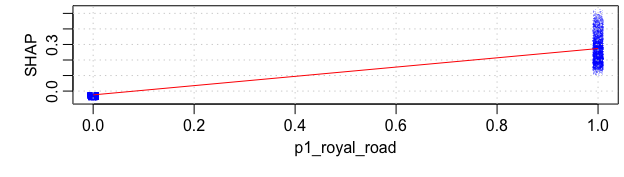
Let’s take a deeper look at royal road and low to high passes. The initial findings for royal road shots are confirmed: there is a big jump in Shapley value when the pass is royal road. In general, almost all shots are improved if the royal road info is added, some dramatically so.

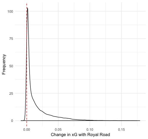
We can see this even more clearly if we pair each shot with and without a royal road pass and plot their actual xG prediction value. To make it viewable, we’ll take a random subsample of 1,000 shots:

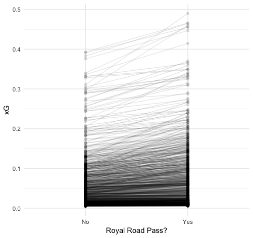
Almost all the shots see some improvement, and some have very steep lines marking a very high improvement in the scoring opportunity.

On the other hand, the results for low to high shots don’t match up with the initial data. Both the Shapley values and the duplicated data suggest that shots are better if they come from a low to high pass than not.

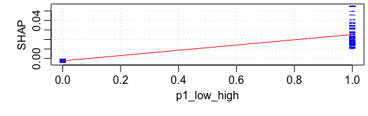
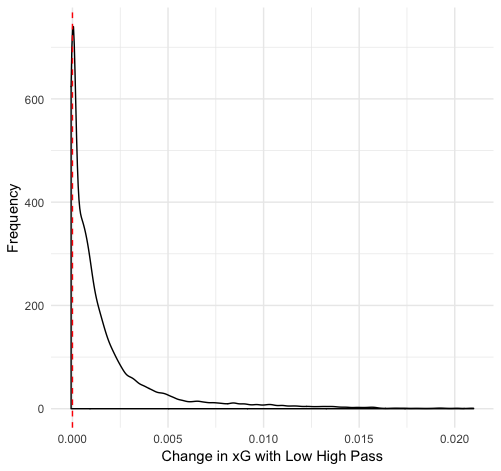
How were we misled by the original dataset? Again, it comes down to collinearity. By design, low to high passes likely lead to shots from the point. These shots are far from the net and particularly unlikely to score, so they’ll generally have low xG values. However, that’s because of the location more than the presence of the pass. If we compare the same point shot with and without the pass, it is better off if the pass preceded it, presumably because it implies puck control sand moving defenders around the zone. That said, the general low value of these plays implies that low to high passes generally don’t lead to success.

With that, we’ve done a decently thorough review of the key new features in the xG model. There’s certainly far more that can be done, but this gives us a general understanding of what features matter and why. The next step is to put them into practice; with better scoring opportunities identified, we need to design systems that encourage players to generate them.

Part 1: Introducing the Model
Part 2: Historic Results and WSH Deep Dive
Part 3: 2018-2019 Results and BOS/S.J Style Comparison