Cowritten by Brendan Kumagai, Mikael Nahabedian, Thibaud Châtel, and Tyrel Stokes

Introduction

This is part one of a two part series introducing our bayesian space-time model for evaluating offensive sequences and player actions. In this part we describe the model and the key metrics derived from it. In part 2 we will show how the model can inform and integrate with player and team evaluations.

Hockey is a game of making the best possible decision in the shortest amount of time. Players need to react quickly to form a chain of plays to create valuable scoring chances. Our goal is to quantify the value of player actions as a function primarily of space and time in the offensive zone. This is to recognize that the puck location and the threat-level it poses to the opposition is a key driver of what options will be available to the puck carrier and – as a result – what is likely to happen next. Ultimately, we want to credit players that are able to make high quality decisions and difficult plays which advance the puck into more valuable locations on the ice.

To this end, we primarily build off of 3 previous papers. First, we use the conceptual framework of understanding play sequences in hockey (Châtel, 2020) from our team member Thibaud Châtel. Second, we adapt the multi-resolutional Expected Possession Value modelling framework pioneered by Cervone et al. (2016) in basketball to work with the detailed play-by-play data generously provided by Stathletes as part of the Big Data Cup hackathon. Finally, using this infrastructure we propose a metric called the Possession Added Value (PAV) based on Karun Singh’s Expected Threat Model in soccer (Singh, 2018) which has previously been adapted to hockey (Yu et al., 2020).

Due to the timeframe of the competition and the complexity of our proposed model, we decided to narrow our scope down to offensive even strength sequences that begin with an entry and end with either a shot or a whistle. By only considering offensive sequences the model as it stands can only properly evaluate the actions of the offensive team.

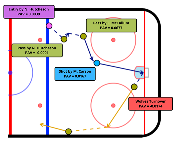
Before we dig into our methodology, here is an example of what our end product will look like in Figure 1 below. We assign each event in this entry-to-exit/whistle sequence with our Possession Added Value (PAV) metric, which can be thought of as the increase in probability that we score in the sequence by performing the observed action. For example, the pass by Landon McCallum from the top of the left circle into the slot adds 0.0677 goals to the expected value of the possession.

The main idea to get there is to build a time machine… well… a hypothetical time machine, not quite a DeLorean with a flux capacitor. 

Let’s look at an example to explain what we mean by this. Suppose we observe an action at the blue dot in figure 1. How would we know how valuable being in that location in space and time is? Now suppose that a player took a shot from there. How would we know if that was a good decision? How valuable is taking that shot compared to say taking a pass?

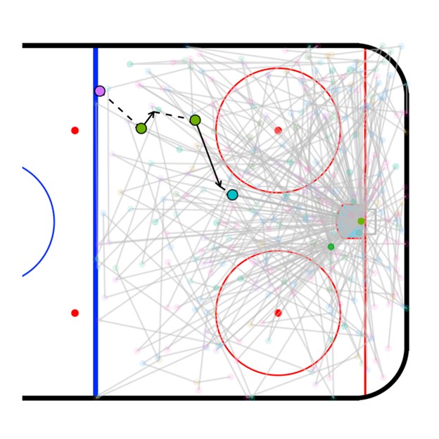
In a perfect world, we would simply recreate all of the exact circumstances of the event and replay it over and over again with an actual time machine. Each time that we replay the event, things won’t happen exactly the same – sometimes we might shoot and score other times we might pass for a one-timer and rebound. We can think of each replay as a possible timeline or path.

Since we can’t actually build a time machine we are going to make a model which is capable of recreating (or simulating) likely sequences – as represented by the grey lines in figure 2. To determine likely sequences we use all of the information available prior to a particularly action which can include the following as inputs:

• where the player is on the ice
• how long has it been since he entered the zone
• how much time is left in the period, the preceding actions
• various other contextual details in the Stathletes data

We plug all of this information into our time machine and we want to find a way to compare what actually happened with what was likely to happen moving forward from that moment in space and time. Plays that create more value than we expect to see from that location are said to add value and those which create less value than the likely sequences are said to decrease value.

Methods

With an overview of what we’re trying to do laid out, we will walk through our five step process in order to determine the offensive value of events through building an ensemble of models that can be used to simulate sequences and estimate the expected value added to the possession by any observed action. Our process will go as follows:

1. How do offensive sequences develop? (Markov decision process)

The first step in building a model that can simulate sequences is to determine how offensive sequences develop. For example, Entry-Pass-Shot-Whistle is a sequence that can plausibly happen, but Shot-Pass-Entry-Entry-Entry-Pass-Exit is not quite as reasonable.

In order to determine how an offensive sequence develops we use a Markov decision process as shown in figure 3. This can be thought of as a flowchart that determines the rules for what actions are possible at different points in the sequence. Each box represents the event that just occurred and the arrows leading out of it represent reasonable transitions to what will occur next.    

Additionally, we have three possible end events: whistle, exit, and goal. If the sequence hit a whistle or an exit, then the offensive sequence will end there. However, goals are a bit more complex, we don’t actually treat goals as a binary 0 or 1 end state, but we use it to store the value of our sequence. We will elaborate further on how we treat goals in Part 4 of the Methods section.

2.How do we determine which event will occur next in a sequence? (transition probabilities & INLA)

Now that we have a nice framework for how offensive sequences can develop and the rules for what actions are possible at different points in the sequence, we need a way to probabilistically determine what is likely to come next.

Figure 5: Possible event flow following a recovery

The most important variables in all of our models are x and y coordinates of the events – in other words – our spatial structure. Defenses are designed to guard valuable space and offenses and offensive players are looking to gain valuable space. In accordance with value as well as the geometry of the rink we expect different actions to be likely in different parts of the ice and across time. But how do we actually model this? 

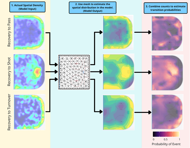
Consider the example of estimating the transition probabilities following a recovery. The Markov decision process flowchart in Figure Y highlights all 3 possible events following a recovery – a shot, a pass, or a turnover. Our model’s main input is where actual observed events occurred following a recovery in the data, represented by the 3 density heat maps in Figure 6.1. Using these 3 sets of data we make 3 different models for the counts or frequency of those transitions actually happening as shown in Figure 6.2. Once we have models for the counts, we follow Cervone et al (2016) by combining the models using the so-called Poisson trick (Lee et al., 2017) to get the probability of transitioning to any of the 3 actions in Figure 6.3. 

These models, as well as all models for this project, are fit in INLA. Below are 6 important steps and considerations for fitting the space-time models we used in this project.

A) Specifying a Mesh: We discretize the ice into discrete triangles as seen in Figure 6.2 and we represent each point on the ice as a weighting of the nearest three nodes. This allows us to reduce computation significantly while still preserving the continuous nature of the ice.

B) Sharing information across the ice: We expect locations near each other to behave similarly and use something called a Matérn covariance function to structure how much information is shared spatially. There are two important parameters, one which determines the range (distance) over which information is shared and the second which determines how noisy the spatial field is.

C) Priors: Bayesian models require priors and the most important for this model are those we put in the Materv covariance function parameters. We use something called penalized complexity priors (Simpson et al., 2017). The idea is that a model which shares lots of information across space with little noise is relatively simple and a model which varies greatly over space with lots of noise is quite complex and our prior penalizes the complex end of the model spectrum. This is a form of smoothing. We can still fit complicated models, but the penalty must be paid in data or information without which the model prefers simpler structures.

D) Sharing information over time: As the play develops from rush to extended zone possession we expect defensive structures to change and thus the options and probabilities of transitioning should change as well. We can take this into account by allowing the maps we build to evolve over time since entry. We share information across time, much like space, by assuming places closer in time are more similar. This is structured formally by putting AR(1) process on the map coefficients, which lets us estimate the correlation over time.

E) Covariates – We can add non-spatial or non-temporal covariates into our model as well, things like score effects or even team effects data permitting. Efficiently adding covariates can be challenging computationally however. The most interesting would be to use the players making the decision to impact the transition probabilities. This is possible using a hierarchical structure to share information across players and player types, but difficult in practice and computationally expensive. However, it is in theory possible and for a good example where this was done with full tracking data see Cervone et al (2016).

F) INLA: We fit these models using Integrated Nested Laplace Approximation (INLA) (Rue et al. ,2009) in R-INLA. INLA is a way to do very fast approximate Bayesian inference for a restricted class of models. This class is called latent gaussian models which includes among others GLMs, GLMMS, GAMs, GAMMs, and even the space-time models used in this paper.  How exactly INLA achieves the speed is beyond the scope of this article. (For more information, there are two nice online textbooks, here and here, and a good overview talk by the principal author.)

3.How does the spatial, time, and contextual information develop? (space/time/context models)

All together steps A through F of the previous section give us a recipe for building our transition probability models. 

However, if we want to put an entire time machine together we need more than just predictions for the next event, we also need to glue all of the events together and tally the value of each of these predicted sequences. 

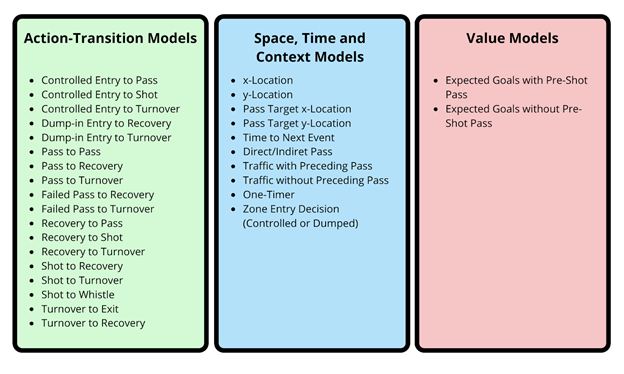
Figure 7 shows all of the models necessary to put the entire time machine together split into three categories. The first of which predict the subsequent action probabilities as previously described in Methods Section 2. The second group predicts where in space and time the play will go to next as well as any covariates which change over time such as whether there is traffic in front of the net. And finally, our expected goals models which value the shots being taken. All of these models use INLA and broadly follow the same process described in Section 2.

4.What is the value of a sequence at a particular moment? (xG models, xPV, and simulations)

With all of these Bayesian models for event-transitions and contextual information complete, we can now tie everything together to build our time machine. Our goal in this step is to quantify the offensive value of a sequence at a particular moment using this time machine. 

For example, given we are at the green point in Figure 8 below, we run simulations to get possible outcomes for how the sequence will develop moving forward as represented by the grey lines.

(Note: the solid grey lines are 10 randomly highlighted sequences to provide a better intuition of what happens in these simulations, while the faint grey lines underneath are the rest of the sequences)

In order to estimate the value of each simulation, we keep track of the expected goals (xG) throughout our hypothetical sequence. 

The simplest route to do this would be to just tally the cumulative xG of each sequence. However, in theory, if a simulation generates multiple high-quality shots then the sum of xG can eventually climb above 1, which is not possible in reality. In effect, this uses xG as a cumulative measure and not as a probability. 

The solution is to treat goals as a branching state. For each shot we take, we know that the xG of the shot is the probability that we score on the shot. Conversely, we would expect not to score with a probability of exactly (1 – xG). Thus, for each shot, we treat the simulation as breaking off into two branches: (1) we score on the shot and the sequence ends with probability xG, (2) the shot is saved and we continue playing with probability 1 – xG. 

As an example, let’s say we are simulating forward from a pass. One possible sequence of events following this pass could be to shoot, recover the rebound, shoot again, then get a whistle. 

In this case, we store the full xG of the first shot – let’s call this – then down-weight the rest of the sequence by , this accounts for the probability that the sequence already ends in a goal after the first shot. Therefore, the value of the second shot will be stored as , which is the probability that we reach the second shot and score on it. Furthermore, if we had n shots in the simulated sequence, the value added to the sequence by the nth shot would be .

By tallying the xG of each simulated sequence in this fashion, we can define the Expected Possession Value (xPV) as the probability of scoring in the rest of the sequence and express it as follows. 

Where is the Expected Possession Value at a moment n with spatial information , at time , and with contextual information and is the expected goals in the ith shot of the simulated sequence. Moving forward will be used to represent for simplicity.

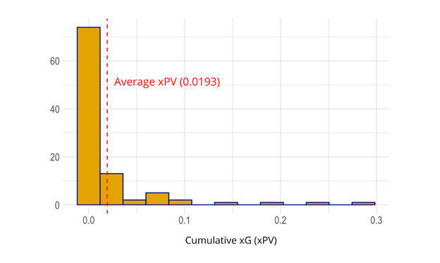
For each simulation run we store the xPV building a distribution for the value at a given point as shown in Figure 9. The distribution of values represents the total model uncertainty of value at that point which we will later use to quantify the uncertainty in our player metrics. For example, in Figure 9 we see that the average xPV of the sequence at the moment shown in Figure 8 (green point above) is 0.0193, however, there are rare cases where we are able to gain up to 0.3 xPV moving forward. 

5. How much value does an event contribute to the offensive potential of a sequence

Now that we can determine the value of a sequence at any observed moment, we can move on to our main goal of determining how much value an event contributes to the offensive potential of a sequence.

In order to do so, let’s walk through an example of how we value a shot from the high slot. To determine the value of this shot we need three things:

a.) The xPV at the moment prior to the shot

b.) The xG from taking the shot

c.) The xPV at the next observed moment following the shot

Upon calculating these three quantities, we can plug them into the following formula to produce the ‘Possession Added Value’ or PAV of the event.

Here, represents the probability of scoring off the shot, represents the expected possession value given that we do not score and represents the expected possession value at the moment prior to taking the shot.

This equation can be thought of as the opportunity cost of executing an action where the positive components, 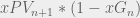(probability we score on the shot) and (xPV of the sequence, given we don’t score on the shot), are the value gained from executing the shot and the negative component, , is the value we no longer have because we took the shot.

There are a few additional edge cases and wrinkles. When the sequence ends following a shot (i.e. shot is followed by a whistle or a goal), we build an additional spatiotemporal model to predict what the xPV would have been if the play were to have continued through a rebound. This ensures we are not undervaluing these cases relative to shots that are followed by a rebound where we include the xPV following the shot. 

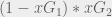
In cases where our observed action is not a shot, we set the xG = 0, which allows us to simplify the equation as follows:

Further, in cases where the following event is an exit, we set , which again allows us to simplify to just:

Conclusion

We have introduced a framework for assigning value to events in the context of offensive zone sequences which consists of two parts building on previous work in Hockey, Basketball, and Soccer. First, we outline the blue-prints to design a time machine for simulating play sequences with modern bayesian space-time techniques. Second, we show how one can use those sequences to meaningfully value space on the ice and actions taken by players.

In part 2 we build off of this work and take a deeper dive at applying the insights from the model and metrics and show how one might integrate this with a comprehensive player and team analysis.

Bibliography

Cervone, Daniel, et al. “A multiresolution stochastic process model for predicting basketball possession outcomes.” Journal of the American Statistical Association, vol. 111, no. 514, 2016, https://www.tandfonline.com/doi/abs/10.1080/01621459.2016.1141685?journalCode=uasa20.

Châtel, Thibaud. “Introducing Offensive Sequences and the Hockey Decision Tree.” Hockey Graphs, 2020, https://hockey-graphs.com/2020/03/26/introducing-offensive-sequences-and-the-hockey-decision-tree/.

Gómez-Rubio, V. (2020). Bayesian inference with INLA. CRC Press. https://becarioprecario.bitbucket.io/inla-gitbook/index.html

Krainski, E., Gómez-Rubio, V., Bakka, H., Lenzi, A., Castro-Camilo, D., Simpson, D., … & Rue, H. (2018). Advanced spatial modeling with stochastic partial differential equations using R and INLA. Chapman and Hall/CRC. https://becarioprecario.bitbucket.io/spde-gitbook/

Lee, Jarod, et al. “On the ‘Poisson Trick’ and its Extensions for Fitting Multinomial Regression Models.” Arxiv Pre-Print, 2017, https://arxiv.org/pdf/1707.08538.pdf.

Rue, Havard, et al. “Approximate Bayesian inference for latent Gaussian models by using integrated nested Laplace approximations.” Statistical Methodology, vol. 71, no. 2, 2009, pp. 319-392, https://rss.onlinelibrary.wiley.com/doi/10.1111/j.1467-9868.2008.00700.x.

Simpson, Daniel, et al. “Penalising model component complexity: A principled, practical approach to constructing priors.” Statistical Science, vol. 32, no. 1, 2017, pp. 1-28, https://arxiv.org/abs/1403.4630.

Singh, Karun. “Introducing Expected Threat (xT).” 2018, https://karun.in/blog/expected-threat.html.Yu, David, et al. A comprehensive analysis of pass difficulty, value and tendencies in ice hockey. ISOLHAC Talk. ISOLHAC Session 3, 2020, https://www.youtube.com/watch?v=Q-kWb6Vshmo.

Yu, David, et al. A comprehensive analysis of pass difficulty, value and tendencies in ice hockey. ISOLHAC Talk. ISOLHAC Session 3, 2020, https://www.youtube.com/watch?v=Q-kWb6Vshmo.