Aggregate statistics in sports have always fascinated me. I might go so far as to say my need to better understand how these metrics work is one of the reasons I became interested in sports statistics in the first place. I also feel the process of developing them raises an incredible number of important questions, especially with a sport like hockey. Rarely are these questions raised in a more succinct and blunt manner than when a new aggregate stat first emerges and people see how good Oscar Klefbom is.

These questions mainly focus on how to value, weight, and interpret the various metrics that are available. For instance, should we value primary points per 60 more than relative Corsi for/against? How much more? Is there a difference? What’s the difference? Should we use some sort of feeling or intuition to determine which stats we like best? How do we address the issue of different metrics being used in conjunction to evaluate players? There have been multiple attempts to “answer” these questions (and many others) in hockey – Tom Awad’s Goal Versus Threshold (GVT), Michael Schuckers and Jim Curro’s Total Hockey Rating (THoR), Hockey Reference’s Point Shares, War-On-Ice’s (A.C. Thomas and Sam Ventura) WAR/GAR model, Dom Galamini’s HERO Charts, Dom Luszczyszyn’s Game Score, and most recently Dawson Sprigings’ WAR/GAR model… (Emmanuel Perry is also in the process of constructing a WAR model that I’m very excited about).

I am a fan of any metric that attempts to combine the disparate aspects of any sport into one number. This fandom started with baseball: wOBA, wRC+, FIP/xFIP, wRAA, UZR, DRS, WAR, etc. One of my favorite aspects of baseball’s various WAR models is that the individual metrics included are (more or less) stats that the average baseball fan is familiar with. When you get down to the guts of the FanGraphs’ WAR calculation (or any of the others), a good portion of it is relatively simple. Baseball, as has been noted many times by beleaguered hockey analysts, is much easier to isolate and measure than hockey. Because of this, baseball’s run expectancy model (the basis for the hitting component of WAR – RE24) is rather easy to understand.

On the other hand, I feel Sprigings’ WAR model has received some criticism simply because people don’t understand how it is constructed. Almost every component is the result of some sort of regression model or machine learning algorithm, so it’s very difficult to interpret or explain the inputs and outputs in a way that makes sense to the average hockey fan. This is not a knock on the model in any way; it’s actually quite the opposite – there’s an inherent presentation issue when using such advanced techniques (explaining it properly feels like reading a statistics textbook).

With that said, Sprigings’ made an interesting note in part 3 of his WAR write up that stuck with me:

“A linear regression would allow a greater insight into the exact influence of each metric included in the regression. I … encourage the public to try and improve on the methodology I have laid out here.”

There hasn’t been anything published that attempted this since so I thought I’d give it a go. Mind you, Sprigings (and many other people) are much more accomplished statisticians than I, but you have to start somewhere. What follows is my attempt to create an aggregate hockey statistic using “well known” metrics and linear regression. It is not perfect. It is not the end-all-be-all. It is not the end of the discussion, and there is definitely room for improvement. But, I feel combining multiple aspects of the game into one number can be insightful and extremely useful (and fun). Additionally, I am a strong proponent of replacement level as a theory in sports statistics, and I feel it has not been utilized or explored enough in hockey. So after I lay out my methodology for constructing the model (part 1), I will adjust the baseline from “above average” to “above replacement” (part 2).

Methodology Intro

First, I think it would be beneficial to familiarize everyone with the method I will be using to create an “above average” statistic. As A.C. Thomas focused on in his Road To WAR series, the baseline for an aggregate stat is very important. I will start by using average (0.0) as the baseline for this metric, and in Part 2 I will transition to “replacement level.” With that said, let’s work through converting a counting statistic to an “above average” equivalent.

To start, I’ll borrow some methods from baseball and create a “points above average” metric to measure a player’s points above (or below) average for each season. To arrive at this number, we need to calculate the average points per minute for each season per position (Forward Total Points / Forward Total TOI, for example) and calculate how much better a player was than league average per minute. We then multiply the per-minute difference by each player’s Total TOI to arrive at Points Above Average (PAA). Here’s what that looks like:

PAA = ((Player Points / Player Total TOI) – NHL Position Points Rate) * Player Total TOI

To demonstrate, here’s the calculation for Ovechkin’s ’08-09 and ’09-10 seasons:

Ovechkin ’08-09 PAA = ((110 / 1803.43) – .0333) * 1803.43 = 49.9

Ovechkin ’09-10 PAA = ((109 / 1555.46) – .0321) * 1555.46 = 59.0

We can see that the 109 points Ovechkin put up over 1555.46 total minutes in ’09-10, using this method, is significantly better than the 110 points he put up over 1803.43 total minutes in ’08-09. This is a result of Ovechkin’s performance per minute in ’09-10, which was significantly higher than ’08-09. This technique is a “counting” stat, but TOI affects the outcome significantly – it’s really more of a “hybrid” counting method. For example, if Ovechkin had the exact same TOI in ’09-10 as he did in ’08-09 his PAA would be 51.1.

This “above average” method will provide the framework for this entire model. If you would like to read more, I encourage anyone unfamiliar to read fangraph’s excellent explanation of Tom Tango’s Weighted On-Base Average (wOBA) and Weighted Runs Above Average (wRAA) – here and here.

Methodology

It’s not normally portrayed this way, but hockey “points” is an aggregate stat – one where goals and assists each have a weight of 1. This is similar to OPS in baseball (where on-base % and slugging % are simply added together). But like baseball, the obvious question is: is that “right”? Are goals and assists equal? What about primary and secondary assists? What about shots? A player’s shot differential? Faceoffs? How do we determine the “value” of these metrics in relation to one another? These questions are similar to those Tom Tango asked when he constructed wOBA.

The weights (or “linear weights”) used in wOBA are essentially derived from the run expectancy of each type of plate appearance outcome (single, walk, home run, etc.) during each type of plate appearance (8 base states, 3 out states). Fortunately for baseball, all of the plate appearance outcomes are well-known measures by themselves and each has a direct (and measurable) impact on run scoring. Unfortunately for hockey, this approach is almost impossible to adapt directly – among many issues, there are exponentially more ways to score or influence scoring in hockey. Because of this, we’ll need to look in the opposite direction: rather than finding the average outcome of prior events, we’ll need to look at the correlation with an “alternate” set of events. The easiest way to do this is by using the split-half regression technique most recently used in hockey by Matt Cane in his Weighted Shots model. There are other ways to perform this type of analysis but, as I mentioned above, they resemble Sprigings’ and Thomas/Ventura’s WAR models and are often difficult to interpret.

This “split-half” technique involves dividing each player’s games (and the respective “well-known” stats) into even and odd game-groups for each season. This provides two samples with which we can perform regressions using the various individual statistics as independent and dependent variables. Additionally, as Matt Cane wrote, “Since there’s nothing in the game number that would relate to our results, if we see a high correlation it’s a good sign that what we’re observing is a talent.” As an added benefit, this more or less separates changes in deployment/usage (powerplay time for instance) evenly between the two groups.

Note: Because of data integrity issues with the NHL’s data, I was only able to use data from 2010-2017. Once Emmanuel Perry (huge thanks to Manny for his scraper and xG model) completes his planned updates, I will re-run this regression to include all 10(+) years of data available from the NHL. Based on additional testing with 5 seasons, the impact of additional seasons is somewhat negligible, but more data is advantageous. Also due to data issues, there were ~150 games missing in total (1.9% of all games). This was basically randomly distributed throughout each season and each team – it affected each player evenly. Hopefully in the future I’ll be able to fill in what’s missing and run everything again.

Regression Analysis

This is going to be long. If you would rather skip ahead, I’ve provided some notes along the way. Here is the framework for my methodology:

1. Determine which stats to test.
2. Set up the split-half even/odd player game groups (including identified metrics)
3. Measure “in-season” repeatability of metrics (correlation with themselves)
4. Perform multiple linear regression with on-ice goals as dependent variable and individual metrics as independent variable(s)
5. Determine best model and finalize coefficients/weights

Here are the “well-known” metrics that I identified and used for testing (all metrics included will be “per 60” rate versions)*:

“Offense”

• Goals
• Primary Assists
• Secondary Assists
• Shots on Goal
• Individual Corsi (shots + blocked shots + missed shots)
• Tango Shots (iCF – Shots on Goal) **
• ixG (Emmanuel Perry’s model)
• xFsh% (ixG / iFF)

“Defense”

• Blocked Shots
• Giveaways
• Takeaways
• Hits For
• Hits Against

“Hybrid”

• Relative CF/CA per 60 (score & venue adjusted, On Ice – Off Ice) ***
• Relative xGF/xGA per 60 (score & venue adjusted, On Ice – Off Ice) ***
• Relative GF/GA per 60 (score & venue adjusted, On Ice – Off Ice) ***
• Relative goals, corsi, and xG differential/60 (i.e. rel CF60 – rel CA60) ***

* Playoff games were not included

** I have affectionately named “non-goal shots” Tango Shots after Tom Tango’s original weighted shot metric for hockey

*** Relative shot differentials are from 5v5 play – all other metrics will be from All Situations (this includes empty net situations and overtime). I will cover my reasoning for not separating strength states later in the article. I will be using Micah Blake McCurdy’s score and venue adjustment for the relative shot metrics

Note: I was not able to incorporate a quality of teammate aspect into this metric at this time. I feel Emmanuel Perry’s method of accounting for QoT is probably the best available, but I was not able to incorporate it into my testing. I hope to be able to adjust for teammate strength in the future. Additionally, I feel the verdict is still out on Quality of Competition (here and here), and, as a result, I will not be adjusting for QoC at this time.

Note: Penalties taken, penalties drawn, and faceoffs will be included as well. I will cover these later.

Now that I’ve laid out the metrics, let’s move to Step 2: in-season repeatability (i.e. Goals.even ~ Goals.odd, etc.). Only “qualified” players were included and forwards and defensemen were separated. I define a “qualified” player as any forward who played at least 4.6 min Total TOI per team game and any defensemen who played 6.0 min Total TOI per team game. This is my way of estimating the top 390 forwards and 210 defensemen from each season (top 13 forwards and 7 defensemen from each team per season). Since the regressions are per 60 rates, including only qualified players allows us to avoid excess variance in rate stats due to limited TOI.

The relative metrics were calculated by taking a player’s on-ice shot metric minus his off-ice shot metric. There are problems with this version of relative shots – mainly, as I noted, with regards to quality of teammate. Hopefully in the future I will be able to explore more advanced “relative” shot metrics in future iterations of this model (i.e. Perry’s article linked above, Dom G’s shot generation/shot suppression model – similar to Sprigings’ XPM – or maybe something similar to Stephen Burtch’s dCorsi model).

Below are the in-season correlations (R^2 values) for each metric I listed above:

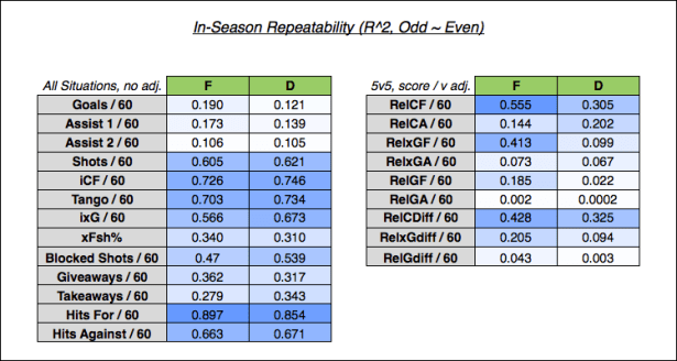
Keep that information in the back of your mind and let’s move on to Step 3: multiple linear regression using on-ice goals. For this step, I used the same technique employed in the “in-season” regression above, but the dependent variable was changed to the opposite group on-ice Goals/60 (either for, against, or differential) rather than the opposite group equivalent (G60.even ~ G60.odd is changed to On-Ice G60.even ~ G60.odd + …). Additionally, this will be a multiple linear regression rather than a simple linear regression (see here if unfamiliar). This multiple regression will be run twice: once with the even group on-ice goals figure as the dependent variable and once with the odd group on-ice goals figure as the dependent variable. Here is what that looks like:

on-ice G60.even ~ G60.odd + A160.odd + A260.odd …

on-ice G60.odd ~ G60.even + A160.even + A260.even …

This produces outputs for each regression that look something like this (this is a simplification and these are fake numbers):

Coefficients:	Estimate	P-Value
Intercept =	0.64	< 0.00000 …
G60 =	0.55	.032…
A160 =	0.69	0.0000 …
A260 =	0.45	0.0000 …
(metric)	(n)	(n)

Multiple R^2

0.36

The coefficient for each regression will be averaged, and the weights for the model will (eventually) be determined.

Process

Note: If you do not want to read my long-winded explanation for how I determined the final metrics that will be included, please skip to the “Regression Results” section.

First of all, this is a balancing act – we want to find the right combination of metrics that are repeatable and impactful on a player’s on-ice goal differential (with a relatively high degree of confidence). I started by running regressions for every combination of independent variables (even/odd G60, A160, A260, etc.) against every combination of dependent variables (odd/even On-IceGF60, On-IceGA60, and On-IceGdiff60). There are two dependent variable options that I tried (without getting more complicated): correlating a group of “offensive” metrics with on-ice goals for and correlating a group of “defensive” metrics with on-ice goals against -OR- correlating a group of all metrics with on-ice goal differential.

Note: It is possible to determine the dependent on-ice goals variable using a regression. This can account for the effects of venue, goaltender, etc. (this is the method used in basketball’s various advanced “plus-minus” statistics and Sprigings’ WAR). However, this complicates the model and is somewhat difficult to interpret, so I have opted to stick with raw on-ice goals for now.

Boxscore Metrics

For the “offensive” metrics, I tested multiple combinations of G60, A160, A260, iSF60, iCF60, ixG60, Tango Shots/60, and xFsh%. Multicollinearity is an issue here – meaning some of the independent variables included in the regression are highly correlated with each other. For instance, a player’s iCF60 is highly correlated with iSF60 (R^2 of around .61). This is true for all of the individual shot metrics. This means we wouldn’t want to include each of iSF, iCF, iFF, and ixG in the same regression, for instance. With that said (and after a lot of testing), I found including goals, primary assists, secondary assists, Tango Shots, and ixG to be the most stable model while avoiding excess multicollinearity. Goals, primary assists, and secondary assists all have a very good correlation with onGF60, and iCF and ixG were the individual shot metrics with the best correlation with onGF60. I used Tango Shots per 60 instead of iCF to decrease multicollinearity – this also prevents “double counting” shots that result in a goal, which is advantageous for both the regression and the actual player level calculation.

The “defensive” box score metrics (iGVA/iTKA, iHF/iHA, and Blocked Shots) were much more difficult. Using on-ice GA60 as the dependent variable, the forward and defensemen models returned an average multiple R^2 between .04 – .08 with only iBLK, iHF, and iHA being within 95% confidence. Additionally, the coefficients are a bit problematic. Regardless of which dependent variable I used (GA60 or Gdiff60), blocked shots had a negative correlation with goal differential – average coefficients of .14 and .09 when correlated with on-ice GA60 (forwards and defensemen respectively). This means an increase of 1 iBLK60 indicates an increase of .14 and .09 of a players on-ice GA60. The same “opposite results” were true with giveaways / takeaways and hits for / hits against – giveaways and hits against are negatively correlated with on-ice GA60, and takeaways / hits for are positively correlated with on-ice GA60. While these results are interesting (and line up with previous work), I feel “punishing” players with a high rate of blocked shots, takeaways, etc. is not ideal. There are a lot of factors at play here that I am not accounting for (team strength and quality of teammate, for example), and the multiple R^2 is low enough that it’s hard to say these metrics even impact on-ice goals against to a significant degree.

Sprigings’ came to a similar conclusion and opted to use a different dependent variable for his model (defensive XPM was used instead of actual goals), but since I am sticking with raw on-ice goals, I do not have this option. These metrics are fairly repeatable, but they don’t correlate well with on-ice goals against or on-ice goal differential so I will be omitting them. This is not ideal, but hopefully the relative shot differentials will provide a better way to assess individual skater defense…

Relative Shot Metrics

Surprise! Properly measuring skater defense is hard (as most people already know). The relative shot metrics regression proved to be to just as difficult as the defensive box-score regression. Based on the repeatability and correlation with on-ice goal differential, relative goals is a terrible metric. This played out in my initial test of on-iceGdiff60 ~ RelGdiff60 + RelCdiff60 + RelxGdiff60 where the multiple R^2 was .02-.04 and relGdiff60 had p-values ranging from .48 – .55 for defensemen. Surprisingly, relxG is also not great. In fact, when only rel Corsi and rel xG were included as independent variables, xG consistently came up with a negative coefficient (again the confidence of this projection is below the 95% threshold for defensemen).

There are also multicollinearity issues when including multiple relative shot metrics in the same regression. They are relatively highly correlated with each other (rel CF and rel xG have an R^2 of .62 to .68), and the model ultimately produced a result that essentially zeroed relative xG differential (and when applied to each player, a higher relxGdiff meant a lower overall total). Not ideal.

I tried separate regressions using on-iceGF60 and GA60 as dependent variables; however, as you may expect from the repeatability table above, skaters have much more direct impact on their on-ice goals for than their on-ice goals against. This resulted in an unequal weighting of the relative for and against numbers, which I feel is not usable. In my mind, a +10 rel corsi/60 is the same regardless of how a player achieved that differential (for instance, 15 relCF60 // 5 relCA60 or 2 relCF60 // -8 relCA60). Also, and maybe the biggest factor here, I’m not accounting for the goalie behind each player or the strength of each player’s team (I will cover team effects later). Because of this, I feel using on-ice goal differential as the dependent variable is the best option.

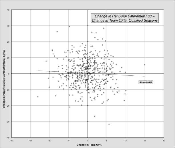
After all of that, and to my dismay, I removed relative xG diff (and relative goals) and was left with the old stalwart that is relative corsi. On-off relative corsi differential is actually pretty repeatable in-season and has the best correlation with on-ice goal differential. After arriving at this result, I looked at measuring team effects on a player’s on-off relative corsi differential. I won’t dive into this too much, but I looked at all players who changed teams from one season to the next. Using this group, I correlated change in relative corsi differential with team CF%. Surprisingly, there was almost no correlation between the two using this sample. I also ran tests attempting to find a connection between a player’s on-ice and off-ice numbers, which yielded nothing. As a result, I will not be adjusting for team strength. Here is what the former test looked like:

 

Regression Results

To summarize:

• The boxscore/counts portion will include goals, primary assists, secondary assists, Tango shots, and ixG. This regression used on-ice GF/60 as the dependent variable.
• The differential portion will include only (on ice – off ice) relative corsi differential per 60 (score & venue adjusted, 5v5). This regression used on-ice Gdiff/60 as the dependent variable.

Here is the initial regression output for the “goals for” regression (G, A1, A2, Tango, and ixG) and the “goal differential” regression (relative corsi differential):

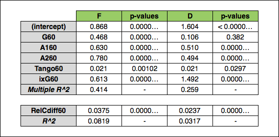
As you can see, we end up with a relatively good R^2 for the box score regression but a rather disappointing one for the relative corsi regression. The box score p-values are very low for forwards and, other than goals (which isn’t surprising) very low for defensemen. It is interesting that, unlike Matt Cane’s weighted shots and Tulsky’s work, secondary assists have a much higher coefficient than goals and primary assists (for forwards). I feel this could be easily misinterpreted, so as an aside, I wanted to illustrate that these weights/coefficients should not be viewed in a vacuum – it is important to look at the frequency of each event being measured. To demonstrate this, here are the per 60 average NHL rates for goals, primary assists, and secondary assists over the last 10 seasons:

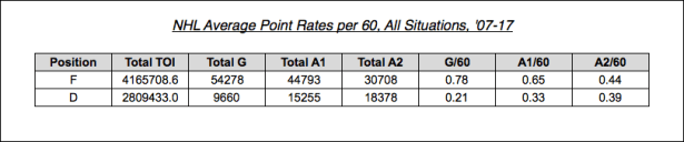
Looking at the forwards, secondary assists have a much higher coefficient than goals (from the regression table) but happen much less frequently. Defensemen are the opposite. If we take the league average rates and multiply them by their respective weights the original linear model produced, we arrive at the following per 60 values:

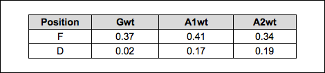
Hopefully, this demonstrates that the coefficients (when viewed by themselves) can be a little misleading. There are a lot of factors at play here. What I can say is that all situations secondary assists appear to be a better indicator of on-ice goals-for than previous even-strength testing has shown. This could be a reflection of better teams recording more secondary assists (leading to a higher goals for rate), or that all situations numbers are different than 5v5. Whatever the reason, it is worth further investigation that I hope to explore in the future. I also hope to be able to account for scorekeeper (venue) effects on secondary assists at a later date, but for now I will not adjust for either of these (potential) issues.

Moving on, based on the suggestion of Dawson Sprigings, I looked into interaction and transforming variables. I tried several transformation techniques, but they provided no significant benefit (this involves, for instance, squaring or taking the square root of one or more of the variables). I also tested using on-ice GF% and something that looks like baseball’s “Pythagorean” win percentage as the dependent variable, but I was not able to discern any obvious benefit so I stuck with on-ice goals.

Interaction variables, however, proved to be very useful. Interaction variables introduce additional independent variables as a way to account for multicollinearity and the effect independent variables can have on one another. As I covered before, Goals, Tango Shots, and ixG have a strong correlation with each other (assists do not have a high correlation with goals or shots so I excluded them from this process). Because of the correlation between the shot components, I added interaction variables to account for the impact of goals on ixG, etc. and vice versa. The new model looks like this:

onGF60 ~ G60 + A160 + A260 + Tango60 + ixG60 + G60* Tango60 + G60* ixG60 + ixG60* Tango60

Running that regression, we end up with the below coefficients:

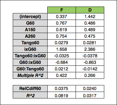
This makes it a little harder to interpret the variables, but you can see the impact. The results essentially show inflated Goals, ixG, and Tango Shots coefficients which are “reduced” by a factor determined by the effect each has on the other. If this gets a little confusing, I will be going through the entire calculation in a bit, so just hold on. Lastly, I used R’s “ridge” package to perform a linear ridge regression instead of the standard multiple linear regression. The linear ridge regression resulted in a model that had a slightly higher repeatability than the multiple linear regression, so I opted for that model (I used the Cule method for setting the lambda parameter which is included in the ridge package). For more information on ridge regression, please see here.

And with that, we have the final coefficients/weights:

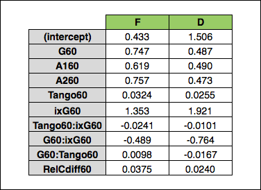
Note: Ridge regression does not output a R^2 value

For penalties taken and penalties drawn, I will use the same goal value that Sprigings uses in his WAR model – one penalty taken or drawn is worth .17 goals:

“The net value in terms of goals of a single penalty is set at 0.17. This comes from the assumption each penalty is worth 1.8 minutes of GF60 going from 2.5 to 6.5, GA60 from 2.5 to 0.73. (6.5-2.5 + (2.5-0.73))*1.8/60 = 0.17”

For faceoffs, I’ll be using all situations faceoff differential and (like Sprigings) Michael Shuckers’ goal value of a +1 faceoff differential. His study found a faceoff differential of +76.5 to equal one goal added. If we turn that around we get a faceoff differential weight of .013 (1 / 76.5 = .013).

Since these coefficients are essentially “predicting” on ice goals for / goal differential, using the above penalty differential and faceoff goal values keeps everything on the same level. The only remaining problem is the strength state of relative corsi differential. Since I am not attempting to account for relative shot differentials at all strength states, I have scaled up the relative corsi coefficient by 75% (divided by 75%) to estimate a player’s relative shot differential during the 25% of the game that does not take place at 5v5 (this is reflected in the table above). I could either scale the weight or scale each player’s 5v5 TOI, but either way we arrive at a similar result.

Arriving at Weighted Points Above Average:

Now that we have our weights, let’s apply them. One of the complications with creating an aggregate statistic for hockey is that some of the metrics are differentials, which adds an additional layer of complexity when combining everything. Because of this I grouped the metrics into 5 components:

• Counts:
  • Goals
  • Primary Assists
  • Secondary Assists
  • Tango Shots
  • ixG
  • [Interaction Variables]
• Differential:
  • Relative Corsi Differential
• Penalties Taken
• Penalties Drawn
• Faceoff Differential

Rather than describing how to use the final weights, I think it would be best to actually show the entire process for how a single player’s final number is calculated. As I stated earlier, I am using a very similar method to how baseball’s wOBA and wRAA are calculated (the same method from the PAA example shown earlier).

Note: I will be ignoring the intercepts and error values that are normally used in an actual projection. Adding a constant “per 60 value” for each player is not advantageous when playing time is such a large factor. Additionally, including these regression components would require a conversion into an “individual” goals number (similar to basketball VORP). Since I’ve determined I cannot properly account for all aspects of the game (defense), I will forgo this “conversion” and scale the coefficients to resemble point totals for each position. This will be covered a little later.

First, each player’s raw totals for each category (goals, assists, etc.) are multiplied by the respective weight and summed to come up with the raw total for each component (counts, differentials, etc.). The coefficients can be multiplied by a player’s raw totals or multiplied the per 60 rates and “expanded” using the respective player TOI figures – either way you arrive at the same number. I will use Connor McDavid’s ’16-17 season to demonstrate (note – these are the “scaled” weights for each season which I will cover shortly):

Counts:	(30*.732) + (44*.607) + (26*.741) + (391*.0318) + (30.37*1.326) + ((391 + 30.37)*-.0236) + ((30 + 30.37)*-.479 + ((30 + 391)*.0096) = 85.81
Differential:	199.49*.0368 = 7.34
Penalties Taken:	-(12*.167) = -2.00
Penalties Drawn:	51*.167 = 8.52
Faceoffs:	-110*.0127 = -1.40

Note: Penalties Taken was turned into a negative – this doesn’t need to be done here – just remember that taking more penalties is not a good thing.

 Every player’s component total (counts, differentials, etc.) is then summed for each season (for each position) and divided by the total TOI to find the league average per minute for each component (the rate tables will be available in the Google doc provided at the end of Part 2). Using the average rates, we can perform the “above average” calculation for each component for each player. The results are summed for each respective player and we arrive at the total wPAA. Here is what that looks like for McDavid:

Counts Above Average:	((85.81 / 1718.65) – .02902618) * 1718.65 = 35.9
Differential Above Average:	((7.34 / 1298.2) – .0002630915) * 1298.20 = 7.0
Penalties Taken Above Average:	((-2.00 / 1718.65) + .002080997) * 1718.65 = 1.6
Penalties Drawn Above Average:	((8.52 / 1718.65) – .001912093) * 1718.65 = 5.2
Faceoffs Above Average:	((-1.40 / 1718.65) – .00000026…) * 1718.65 = -1.4
Total wPAA:	35.9 + 7.0 + 1.6 + 5.2 + -1.4 = 48.3

Note: the league rates used above are the average per minute numbers (factors) for forwards from ’16-17

Season Scale

As I mentioned earlier, I will be scaling everything to look like point totals instead of running an additional calculation to arrive at a goal value. I used Tango’s method for scaling wOBA as an inspiration (seen here). I divided the total positive PAA for each season for each position by the total positive wPAA to arrive at the position “wP Scale” for each season (the positive totals are used because the total wPAA and PAA equals zero). The distributions of PAA and wPAA are very similar, so I feel comfortable with scaling in this manner. While wOBA uses one scale, I feel that forwards and defensemen are different enough that scaling each separately is advantageous. Additionally, it allows for an easier comparison with PAA, which could be interesting. Additionally, if you noticed the intercepts above, there is significantly less that is actually accounted for in the defensemen weights (much higher intercept/lower R^2 than forwards), which makes defensemen appear to be less “valuable”. This could be a little misleading, so I opted to scale the weights to mirror real point totals for each season.

Here are the totals so you can see what the scale calculation looks like:

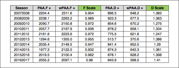
Each weight for each season is then multiplied by the respective scale value shown above for each position. The entire calculation is re-run using the scaled weights to arrive at each player’s seasonally adjusted wPAA. Here are the weight tables for each position so you can see what this looks like (similar to the wOBA table that was linked above):

Forwards:

 

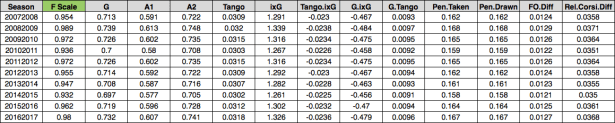
Defensemen:

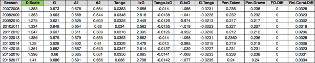
Notes:

At this time I think it’s important to cover a couple things. First, I have not completely accounted for skater defense – this results in a rather offense-intensive stat as I was not able to “offset” the goals-for “box score” regression with a goals-against equivalent. While the “differential” component does provide an aspect of skater defense, it is not equal in relation to the counts component.

Second, I want to explain why I am not breaking out strength states. As you’ve seen above, a below-average number is negative and “hurts” a player’s total wPAA – this is a problem with powerplay time. If I separated strength states, poor powerplay performance would be detrimental to a player’s overall total. The main issue here is usage – or, what do you do with the players who were not given time on the powerplay? Are they “better” because they didn’t play on the powerplay? Well, no, quite the opposite (in most instances). This would introduce a kind of survivorship bias that would require a correction (and that gets very complicated). Additionally, going down this road begs the question: where do you stop with the strength states? Do you separate 6 on 5? 6 on 4? Do you separate 4 on 4 and 3 on 3? The number of strength states in hockey is a hurdle that is not present in baseball or basketball (or soccer for that matter), and the powerplay is something that is wholly unique to hockey as a sport. Because of these issues, I did not separate strength states.

Tomorrow, I will dive into the theory, history, and methods for measuring replacement level, and I will lay out my method for adjusting this model from “above average” to “above replacement”.

Note: All data will be made available at the end of Part 2.