I have written a couple articles over the past few months on using R with hockey data (see here and here), but both of those articles were focused on intermediate techniques and presumed beginner knowledge of R. In contrast, this article is for the complete beginner. We’ll go through the steps of downloading and setting up R and then, with the use of a sample hockey data set, learn the very basics of R for exploring and visualizing data.

One of the wonderful things about using R is that it’s a flexible, growing language, meaning that there are often many different ways to get to the same, correct result. The examples below are meant to be a gentle introduction to different parts of R, but please know that this really only scratches the surface of what’s available.

The code used for this tutorial (which also includes more detail and more examples) is available on our Github here.

Downloading R and Getting Set Up

To use R, you need to download R itself as well as RStudio, which is the main integrated development environment, or IDE, for R. (IDE sounds fancy, but it just means an application where you can run code and actually use the R language.)

• R. The links to download for Mac, Windows, and Linux are at the top of the page: https://cloud.r-project.org/
• R Studio. Underneath where it says R Studio Desktop Open Source License (which is the free version), click download: https://rstudio.com/products/rstudio/download/

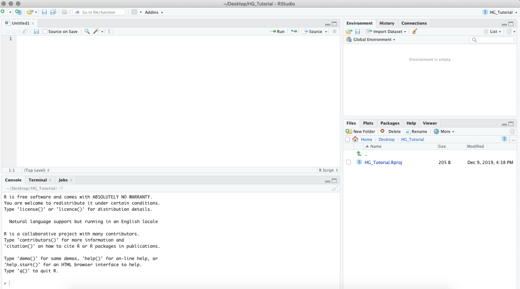
When you open RStudio, it will likely look like this:

The top right section is the environment, which is where all of your data frames and functions will go. The bottom right has several sections: files will show all the available files in the folder associated with your project, plots is where your graphs will show up, packages will list all your installed packages, and help is self-explanatory. On the left is the console, which is where you can run code.

(Don’t worry if you didn’t understand all of those terms. We’ll get there!)

I prefer to do my R work in “projects.” A project generally serves as a folder on your computer where you can keep all of your code and associated files in one place. For example, I have separate projects for my work on goalie pulls and for my work on penalty kills. Create a new project by going to File > New Project.

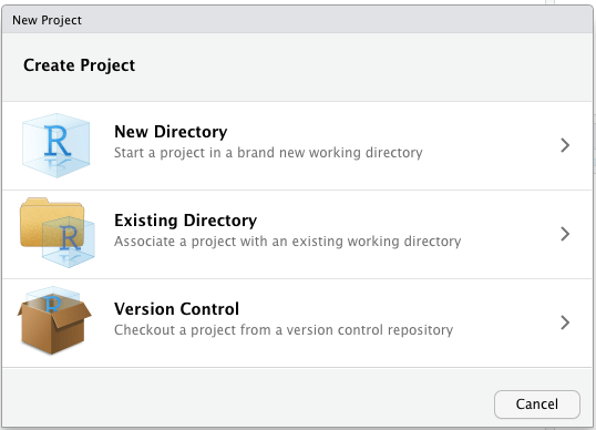
Select New Directory, then New Project, give it a title, and decide where you want the folder to go. My project here is called HG_Tutorial, and in the screenshot below, you can see the title is now at the top of the screen and in the top-right corner.

Once you’re working in a new project, we can open a new script file by going to File > New File > R Script. The script, which will move to the upper left, will serve as a convenient place to write and save all of our code. You can also run code line-by-line in the console, but the script makes it easier to write more code and only run pieces at a time.

Using Packages

There are certain things you can do without packages, in what’s known as “base R.” However, most people use packages to do their work. Think of packages like apps for your phone: there are thousands, of varying quality, that can help you do just about anything you want to do in R. And just like with apps, the typical user spends the majority of the time working with a handful of very popular, well-maintained packages. Once you learn more about R and develop more specific needs, you can search out and use specialized packages.

For this introduction, we’re only going to use one package: tidyverse. The tidyverse (which is actually a collection of packages) is one of the most popular packages and will cover the vast majority of what beginner and intermediate users need in terms of data manipulation, exploration, and visualization. The tidyverse is also well-documented online, which can be very helpful for beginners. If you’re having a problem with something in the tidyverse, I can almost guarantee that someone else has already had that problem and the solution is readily available via Google.

This is how you install the tidyverse (or any other package):

install.packages("tidyverse")

To actually run your code, either place your cursor at the end of the line or highlight a section of code and select Cmd+Enter or Ctrl+Enter.

Once you install a package on your computer, you won’t need to install it again. However, each time you start a new R session, you will need to reload the packages, which you do like so:

library("tidyverse")

It’s common coding practice to load all of the packages at the beginning of your script, so someone reading it knows in advance all the packages they will need. (In general, it’s a good idea to write your code as if someone else will be using it. And “someone else” definitely includes future you in three months, who won’t remember anything from the first time you wrote it.)

It’s also common coding practice to use comments, which you can do by adding # to the front of the line.

# This is the package we're going to load!
 
library("tidyverse")

Writing Your First Code

# Read in our data set and give it a name
 
PHI_tutorial_data <- 
  read_csv("https://github.com/meghall06/HG_Tutorial/blob/master/PHI_tutorial_data.csv?raw=true")

The left arrow shows up a lot in R and is generally used to “assign” something. That is, you’re asking R to do a task and then save the results into an object—often a data frame, which is what we’re doing in the example above. (If we ran this code without the data frame name and the left arrow, R would still do it, it just wouldn’t save the data anywhere, which isn’t very useful.) The keyboard shortcut for this arrow is Alt/Option + -.

read_csv() is a function, and functions are the basis of most of what you do in R. All functions start with their name (read_csv, in this case) and are followed by their arguments in parentheses. The arguments will differ by the type of function, and there are often many optional arguments beyond what’s necessary to run the code. (You can also make your own functions, ranging from basic to advanced, but that’s beyond the scope of this article.) This specific function reads csv files.

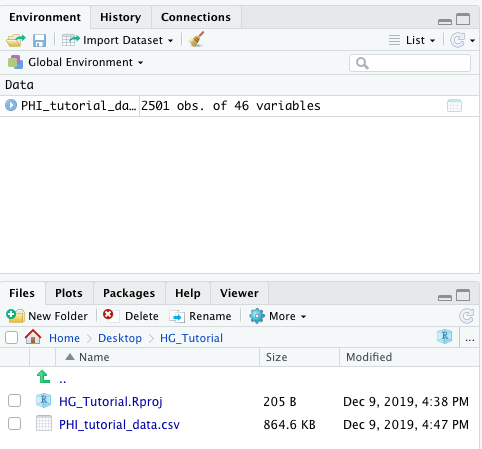
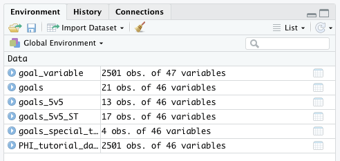
Once we run this code, that data frame we created is available in our environment in the top right corner of the screen. We can see that it has 2501 observations (i.e., rows) and 46 variables (i.e., columns). The code above downloaded the csv from my Github page, but as you can see in my files section at the bottom right, I also have this file saved on my computer. If you’re working with a file within your project, you can use the read_csv() function like this:

# Read in a file from your computer
 
PHI_tutorial_data <- 
  read_csv("PHI_tutorial_data.csv")

Let’s start by taking a look at this sample data set. If you click on the data frame name in the environment section, it will pop up in an Excel-like format. (You can also do this with the view() function.)

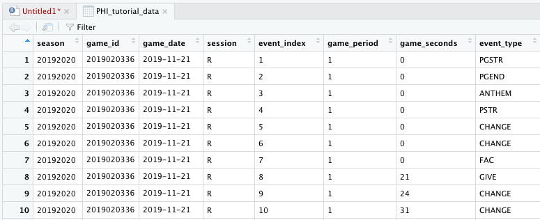
The NHL makes play-by-play data available online, and we can scrape that data into a format that’s easily used and analyzed. This sample data set contains data from four Philadelphia Flyers games last month that I scraped using EvolvingWild’s scraper. (In the full example code available on our Github, I’ll show you exactly how I did that.)

You can explore the data set yourself to see what is available, but in a nutshell, there is one row per tracked event that provides details of that event: what time it occurred, which players were on the ice, etc. Unique identifiers are very important when working with data, and with this data each game has a unique game_id and each event within a game has a unique event_index.

Exploring Your Data

We saw earlier that the left arrow is mostly used to assign things. You can also think of it like “save as” in Excel, where you start with one file and give it a new name, whether or not you make changes to it. We can do something like this, which will simply create a copy of our data frame:

# Copy our data 
 
copy <- PHI_tutorial_data

Or we can “save as” and start to make some changes! It’s generally good practice to save to a new data frame when you’re making changes, particularly at the beginning. This way, it’s much easier to recover if you make a mistake because you still have your original data frame. Let’s create a new data set called goals and filter down to just the goals that occurred.

Filter

# Filter down to just goals
 
goals <- PHI_tutorial_data %>%
   filter(event_type == "GOAL")

In the code above, we created a new data set called goals, using the original data set as our source. We used the filter() function and asked to keep only the observations (i.e., rows) that had an event_type of GOAL. After you run this code, the new data set should pop up in the environment in the upper right. We can see that in these four games, 21 goals were scored.

A couple of comments on notation:

• This symbol %>% is known as the pipe, and it’s an integral part of the tidyverse “language.” You use it to continue your “thought” and indicate that the following line is part of the same code chunk.
• When you’re testing for equality, you must use double equal signs. If you forget, which you definitely will at times, you’ll get the following error in your console:

# Filter to 5v5 goals only
 
goals_5v5 <- PHI_tutorial_data %>%
   filter(event_type == "GOAL" &
            game_strength_state == "5v5")

You can also use multiple conditions in your filter statements. If we were interested in only filtering down to five-on-five goals, we use the & symbol and add in a condition for the game_strength_state variable, as well.

# Filter down to goals at 5v4 or 4v5
 
goals_special_teams <- PHI_tutorial_data %>%
   filter(event_type == "GOAL" &
            (game_strength_state == "5v4" |
               game_strength_state == "4v5"))

The same is true if we wanted to look at special teams goals. In play-by-play data, the game strength state is given by the home team’s strength first, so both “5v4” and “4v5” could be a power play. In R, “or” is indicated by the | symbol.

# Filter to all goals at 5v5, 4v5, or 5v4
 
goals_5v5_ST <- PHI_tutorial_data %>%
   filter(event_type == "GOAL" &
            game_strength_state %in% c("5v5", "5v4", "4v5"))

If we wanted to see goals at all three of those strengths, it’s probably easier to use the %in% notation rather than several “or” statements. It indicates that we only want observations with a game_strength_state variable that matches one of those options. The c() notation just denotes that it’s a list.

Select

# Slimming down the goals data set
 
 goals_small <- goals %>%
   select(game_id, game_date, event_type, 
          event_detail, event_team, event_player_1)

Let’s briefly return to the full goals data set. As you can see in the top right environment, that data set has 46 variables. That’s a lot, and for our hypothetical purpose of seeing which players scored which goals in these four games, that’s more information than we probably need. We can use the select() function to tell R that we want to drop or keep certain variables. There are lots of different ways to do this, depending on how many variables you want to drop or keep, but in this example, we’re keeping it simple and asking R to keep only six variables. (The variables will show up in the order that you specify, so you can also use select() to reorder variables.) Once you run the code above, you can confirm that a new data frame called goals_small appears and has only six variables.

Mutate

# Creating a new data frame with a goal variable
 
 goal_variable <- PHI_tutorial_data %>%
   mutate(goal = ifelse(event_type == "GOAL", 1, 0))

Let’s return to our original data and practice creating a new variable (i.e., column). Let’s create a simple 0/1 variable to determine whether or not each observation represents a goal. Mutate() is the function for creating a new variable, and the new variable name is the first argument in the function. (You can see here that we use a single equal sign for creating a variable instead of a double equal sign because we’re not testing for equality.) To determine if there’s a goal or not, we need an ifelse() statement. The basic ifelse() statement has three arguments: the condition (here, whether or not event_type is GOAL), the result if the statement is true, and the result if the statement is false. We’re telling R that if event_type is GOAL, this new variable should be a 1. If not, it’s a 0.

Generally after you create a new variable, you want to make sure that it worked correctly. In this case, we can check in the top right environment to make sure that the new data frame called goal_variable shows up. It’s there, and we can also see that it has 47 variables (i.e., columns) instead of 46 like the original, which is a good sign.

# Double check that our variable creation worked
 
 sum(goal_variable$goal)

And since our new variable is a 0/1 variable, we can run a quick line of code to sum up all of those 1s. Since we created a specific goals data set before, we already know that there are 21 goals in this data set. The above line of code is a simple summation, using the syntax of dataframe$variable, and when you run it, you can see the correct result of 21 down in your console. (If we wanted to assign this value to something and save it so we could use it again or reference it later, we would have to use a left arrow. But we don’t, we’re just using it to check, so it’s fine that the number is only available in the console.)

# Double check that our variable creation worked with count
 
 count(goal_variable, event_type)

One other way to double-check that this variable is correct is to use the count() function. (You could also use this on its own if you were only curious how many goals were scored and didn’t need to make another variable to use later.) The count() function takes as arguments the data frame (goal_variable) and the variable of choice (event_type) and returns a list in the console of all the unique values and their frequencies of the event_type variable. If you run this code, you’ll see the output in your console, like below, and note that there are 21 goals.

Group and Summarize

We now know multiple ways to find out how many total goals were scored. But what if we’re curious as to which teams scored those goals in which games? To do that, we can use the powerful combination of the group_by() and the summarize() functions. Group_by() allows you to section your data based on one or more variables, and summarize() can apply certain functions to each of those groups separately.

# Use group_by and summarize to find total goals per game
 
 goals_by_game <- goal_variable %>%
   group_by(game_id) %>%
   summarize(total_goals = sum(goal))

The code above will create a new data set called goals_by_game that will group our data set by game_id (the unique identifier for each game) and summarize our goal variable that we created in the last section. That summarized variable will be a new variable that we’ll call total_goals.

If you run this code and look at the data frame, you can see that it has been reduced to just our grouping variable, game_id, and our new summarized variable, total_goals.

# Add event_team so we have total goals per game per team
 
 goals_by_game_team <- goal_variable %>%
   group_by(game_id, event_team) %>%
   summarize(goals = sum(goal))

But what if we also wanted to see which teams scored the goals in those games? Let’s add that variable to our group_by() function and see what happens.

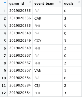
That output is less than ideal because in this case, I don’t really care about those NA values, they’re just cluttering up our output. Why did that happen? If you examine the play-by-play data, there are certain event types that don’t have event teams associated with them (e.g., period starts and ends, stoppages in play), but by adding event_team to our group_by() function, those NA values will show up because they’re a unique value of that variable. Let’s redo this code and get rid of those NA values first.

# Let's try that again and remove the NAs first
 
 goals_by_game_team <- goal_variable %>%
   filter(!is.na(event_team)) %>%
   group_by(game_id, event_team) %>%
   summarize(goals = sum(goal))

We can do that by adding a filter() function before we do our grouping. is.na() is a common function used to identify NA values, and the ! in R means “not.” So this one line of code is telling R to keep only the observations that do not have a NA value for event_team. The rest of the code is the same, and if you run it, you should see the output below.

Arrange

arrange() is a function used for sorting. We don’t particularly need it with this small data set that we’re working with because it’s only eight observations, but it’s very useful for when you’re exploring larger data sets or want to arrange data for presentation purposes.

# Arrange by number of goals
 
 goals_by_game_team <- goals_by_game_team %>%
   arrange(desc(goals))

You can see with the code above that I’m not actually creating a new data frame, I’m just using the left arrow in a “save as” manner and modifying this one data frame. Using the desc() function around our variable of interest will put the observations in descending order, as you can see below, but if you removed that, the default order for arrange() is ascending order.

Making a Graph

The tidyverse package for making graphs is ggplot2, which is very powerful. You can make many different types of graphs and customize them in endless ways, but we’re just going to go over a very basic chart format so you can see the syntax.

# Make a bar chart!
 
 ggplot(data = PHI_tutorial_data) + 
   geom_bar(aes(x = event_zone))

The code above will make a very basic bar chart of how many observations (i.e., events) took place in each event zone. The geom_bar() function indicates which type of chart we’re making, and the “aes” stands for aesthetics. There are many available options here, but here we’re just telling R that we want the event_zone variable on the x-axis. (Note that instead of the pipe %>%, ggplot2 uses a plus sign.)

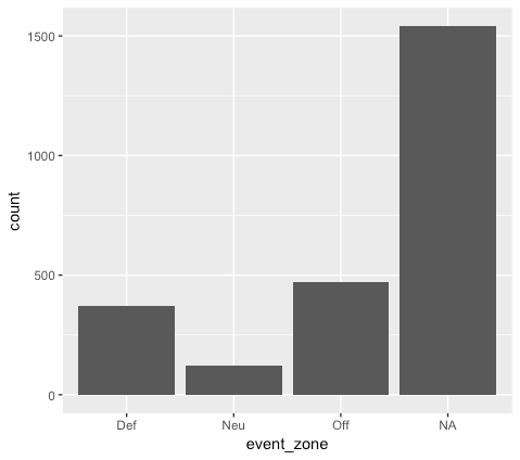
Once you run this code, the plot should pop up in the bottom right corner of your screen. You can save the plot as an image by selecting Export right above it.

# Make a bar chart with some color!
 
 ggplot(data = PHI_tutorial_data) + 
   geom_bar(aes(x = event_zone, fill = event_zone))

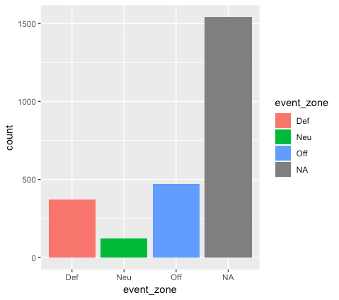
As I mentioned before, there are many other aesthetic options you can add, including “fill,” which will add color based on the variable you select. You can use the same variable like we did here, to get a plot that looks like the one above, or you could use a different variable.

# Add a label to the y-axis
 
 ggplot(data = PHI_tutorial_data) + 
   geom_bar(aes(x = event_zone, fill = event_zone)) +
   labs(y = "Number of Events")

You can also add an axis label, as shown above.

The basis of all ggplot2 code is similar, just using different “geoms” (i.e., we just used geom_bar() to make a bar chart, while geom_point() will make a scatter plot) and different aesthetic mappings. This is a very helpful cheatsheet for ggplot2.

You Made It!

I hope this was a gentle and informative guide to getting started with R. I’m on Twitter @MeghanMHall if you have any questions, and the code is available on our Github here. That code contains everything discussed here, some more details, and also six exercises based on these techniques to help you practice. For further reading, these are a couple of my favorite resources:

• R for Data Science
• RStudio Community
• Tidyverse documentation

And if you’re interested in hockey data specifically, I have written two other articles (here and here) that focus on techniques that are particularly helpful for working with hockey data.

Keep your eye out in the new year for even more content from Hockey-Graphs!