
This work is co-authored with Madeline Gall.
While scouting for some sports is straightforward (college football → NFL), scouting for the NHL can be a more arduous process. With players from over 45+ international ice hockey leagues, each with its own regulations and difficulties, how can one adequately assess the quality of a player’s performance? Comparisons between leagues are not easily made; 18 points for an eighteen year old playing against other eighteen year olds in a minor league should not be attributed the same value as 18 points for an eighteen year old playing against veterans in the NHL.
There have been other attempts to account for this, including player translation variables, like that of Rob Vollman’s hockey translation factors, and Gabriel Desjardin’s NHL Equivalency Ratings (NHLe). Desjardin’s NHLe previously tackled the issue of comparing and predicting player performance for League-to-NHL transitions (moving from another league into the NHL). It was great for a quick, general comparison and certainly has its advantages (easy and quick to calculate), but there are some drawbacks to its method. For starters, it didn’t necessarily control for team quality, position, and age. Translation factors are calculated using statistics from players who have played at least 20 games in the given league before playing at least 20 in the NHL. That means there’s a lot of valuable data about these in-between transitions that aren’t being used.
In this project, we introduce a new method for comparing and projecting player performance across leagues using an adjusted z-score metric that would account for these drawbacks. This metric controls for factors such as age, league, season, and position that affect a player’s P/PG metric, and could be applied to any league of interest. This new metric is necessary as there are many characteristics that vary from league to league. Due to the different playing styles and opponent difficulty, there is not one consistent metric to make comparable evaluations of player performance for hockey leagues around the world. Other factors such as goalie strength, penalty rates, and rink dimensions are also inconsistent across international leagues. Scenarios could occur in which players of similar strength could appear to have seemingly different performances.
One such example of this would be Thomas Harley and Ville Heinola from the most recent 2019 draft. Both are players from different leagues playing against different opponents and putting up vastly different numbers, yet were valued to be approximately the same. Harley, an American-born defenceman playing in the canadian junior ice hockey league, is currently playing with the Mississauga Steelheads in the Ontario Hockey League. He was drafted 18th overall by the Dallas Stars in the first round of the 2019 NHL Entry Draft. Heinola on the other hand is a Finnish professional ice hockey defenceman currently playing for Lukko in Liiga on loan as a prospect for the Winnipeg Jets of the National Hockey League. He was ranked as one of the top international skaters eligible for the 2019 NHL Entry Draft. Heinola was drafted 20th overall by the Jets. How did these two players end up being evaluated by their respective teams? Probably with something similar to our metric in addition to scouting information.
For our metric, we were inspired by not only the previous approaches like NHLe, but also the recent surge of Elo. Elo is a method for calculating the relative skill levels of players in zero-sum games. While initially created in the context for measuring chess player ratings, Elo can be applied in various other scenarios as well, like professional sports. To read more and see examples of Elo in sports, a tutorial by 538 can be found here. Elo is simply a specific model for paired comparison model. We will walk through the process in which we created our paired comparison/Elo model.
To begin, we used a dataset that contained around 300,000 observations from the player information (name, position, league, birthday, etc) and player statistics (games played, goals, assists, etc) that were available, scraped from eliteprospects.com. One of the first issues we ran into was what kind of response variable could we create to compare player statistics, controlling for age, league strength, position, etc. Player performance has been calculated extensively within the NHL; there are various measurements such as WAR, GAR, Corsi, etc. However, data collection is not equal in all leagues. Some leagues were not as proactive about tracking stats like hits and blocks as others, which meant we could only utilize variables that were ubiquitous in all leagues as factors within our regression.
When creating the new response variable, we wanted to transform point per game in a way that accounted for age, season, position, and league. The first step was taking the log of points per game plus one. This transformation had a more normal distribution while raw points per game was very right skewed. Even though the log transformation helped the data appear to be more normally distributed, the log points per game still did not account for the variables listed above. We decided that in order to account for such variables, we were going to create a z-score for each player’s log points per game. The first step was to calculate the mean and standard deviation for each group of position, season, league, and age. Then a z-score was calculated for each player observation using the mean and standard deviation that pertained to the variables we were controlling for. Thus, the z-score of the log of points per game plus one was our final response variable. The z-scores appeared to be even more normally distributed then the log points per game, and the z-scores for groups such as defenders and forwards were also normally distributed.
Creating the paired-comparison model, which is very similar to an Elo model. To begin, we build a comparison dataframe. We create pairs of player-league seasons for each player, so that there’s a small dataframe of all pairwise comparisons for the leagues that they’ve played in. This means that if a player has played in K leagues, then that player will have K-choose-2 pairs of player-league-seasons. Next, we eliminate any pairs that have the same league, as well as pairs that are further than one season apart, and calculate an outcome variable. This variable can either be continuous or binary, depending on the regression used. It is important to understand that the “harder” league to play in would actually have a lower outcome variable. This is based on the assumption that harder leagues have better defensemen and goalies, making it more difficult to score.
| Player Name | League | Season | Z- Score |
|---|---|---|---|
| Kris Letang | QMJHL | 2006-07 | 1.829 |
| Kris Letang | NHL | 2006-07 | 1.158 |
| Kris Letang | AHL | 2007-08 | 1.557 |
| League 1 | Season 1 | Z-Score 1 | League 2 | Season 2 | Z-Score 2 | Z-Score Difference |
|---|---|---|---|---|---|---|
| QMJHL | 2006-07 | 1.829 | NHL | 2006-07 | 1.158 | 0.671 |
| NHL | 2006-07 | 1.158 | AHL | 2007-08 | 1.557 | -0.399 |
| QMJHL | 2006-07 | 1.829 | AHL | 2007-08 | 1.557 | 0.272 |
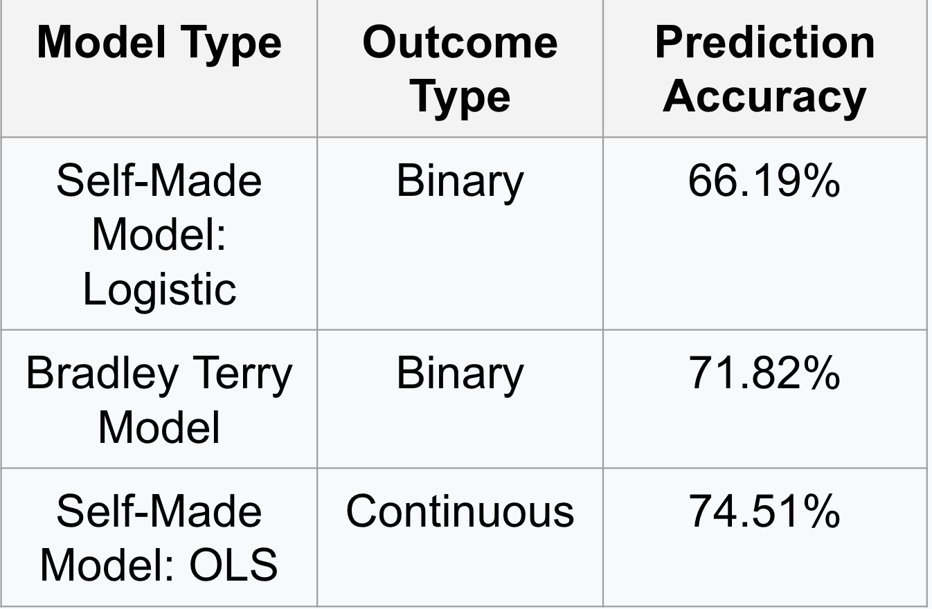
After building the paired comparison model, different types of regressions were used to calculate the coefficients. We focused on using a self-made logistic model, the Bradley Terry model (using the BTm package in R), both which created binary outcomes, as well as an Ordinary Least Squares regression, that created a continuous outcome. To evaluate which regression worked to create the most accurate results, we first split the paired data 70/30 for training and test samples. We then predicted the probability of a win for all the leagues, based off of the adjusted points per game Z-score. A threshold for “winning” was set; if the probability was greater than the threshold, then the predicted outcome was = 1. Otherwise, it was = 0. From there, the predicted outcomes were compared to the actual outcomes to calculate the prediction accuracy for each model. The results are shown in the following table below.
After our different modeling methods were created, we were able to use the strength coefficients from the models in order to create a ranking of leagues determined by their strength. It was no surprise that for each year from 2008 until 2018, and for the overall strength coefficients that the National Hockey League is considered the strongest league. The other league that was consistently considered the second best was the World Championships, which makes sense as these are the best players from different countries competing, and this tournament consists of many players who play in the NHL. Simply looking at leagues, the AHL, KHL, SHL, and DEL were consistently some of the strongest leagues of 45 plus teams. The final ranking of the top 10 leagues were the NHL, World Championship, World Junior CHampionship, KHL, SHL, AHL, USDP, World Junior Championships U18, DEL, and NLA. Some of the leagues that may have been a surprise were the junior hockey leagues, or the USDP. These leagues appeared higher on our ranking because we accounted for age in our model. This allowed the strength to be based on the quality of players rather than the players age. Each of the three models we created had similar rankings with only slight deviations.
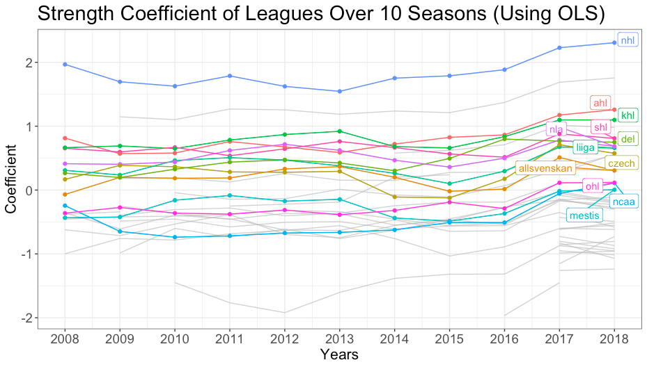
Strength Coefficients Over Time: The above graph shows the strength coefficients for each league for every year from 2008 – 2018. The more commonly known leagues and consistently strong leagues are highlighted above.
After generating a ranking of leagues based on our adjusted points per game, the next step was to see how these rankings compared to using just points per game. When using just points per game we noticed that three things happened to league’s strength coefficients. For leagues that had a higher strength coefficient, those leagues tended to still be the stronger leagues for adjusted points per game. For leagues that were in the middle tier of all of the leagues, their strength coefficients for raw points per game were very similar to their adjusted points per game strength coefficients. Lastly, the leagues with the lowest strength coefficients for raw points per game had worse strength coefficients for adjusted points per game. The only leagues that had lower strength coefficients that had strength coefficients improved by adjusted points per game were leagues that had young players. This trend happens for the World Junior Championships for both U20 and U18, and for the United States High School, Minnesota league. For the Minnesota high school league, it was considered the worst league by far when using raw points per game as the response variable, but by using adjusted points per game, this league performs better than 10 other leagues, many of which are professional leagues. This allowed us to see further the flaws with points per game as a predictor of league strength, and also highlighted how important it is to account for age when determining league strength.
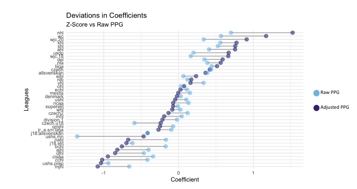
Strength Coefficients for Each League for Raw P/GP vs Adjusted P/GP: This graph displays the strength coefficients for each league for the two different response variables. The strength coefficients were calculated using the same modeling method.
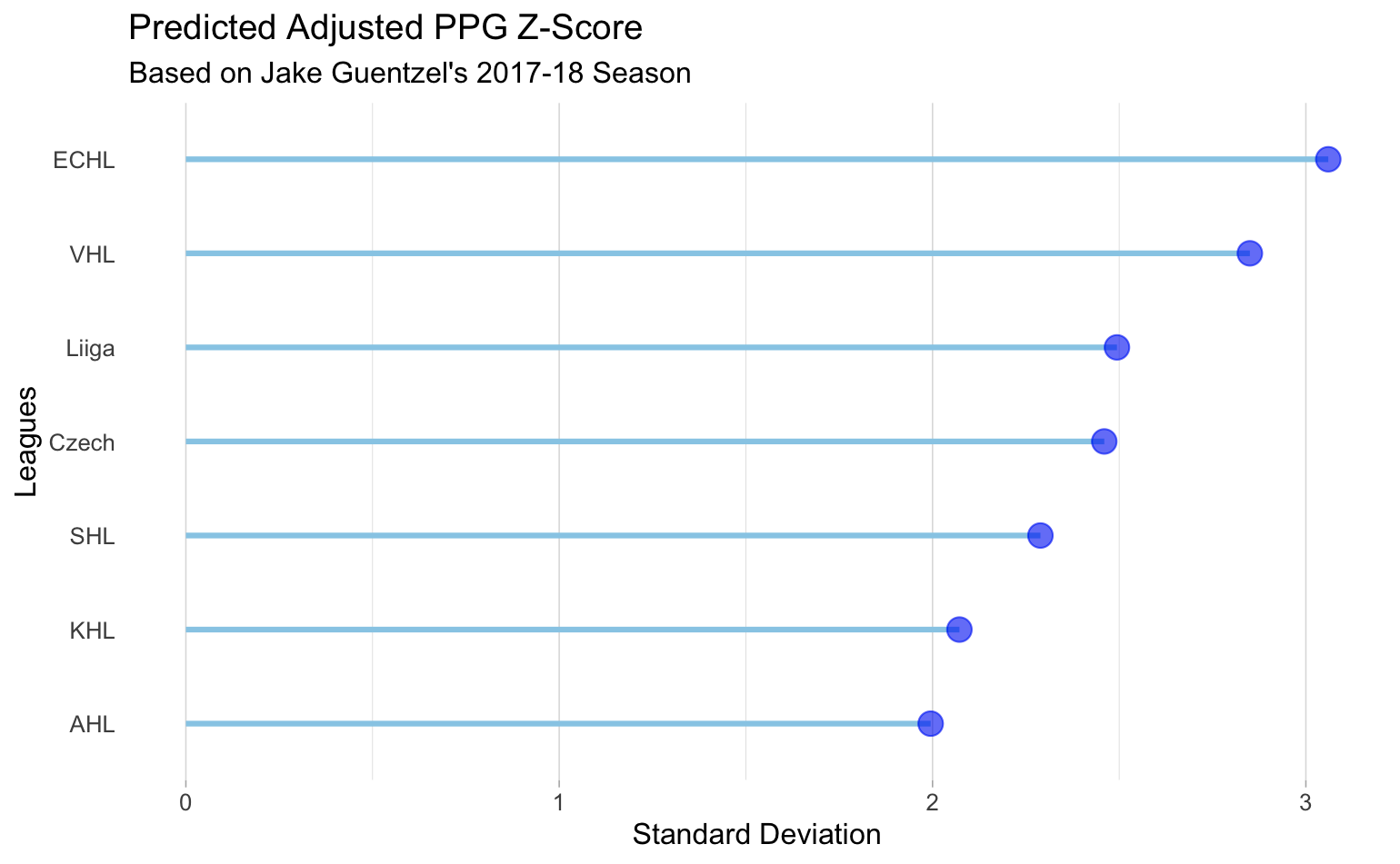
As mentioned above, a new estimate for player performance needed to be created because existing predictors such as points per game are biased due to age, league strength, team strength and the year. Creating percentiles for player types allows a prospect to be compared to other players similar allowing for a more accurate prediction. The percentile of log P/GP and our method chosen is very useful because it allows for a prediction of any given players performance in any of the 45+ leagues. WIth so many leagues, it is not guaranteed that a player would have been drafted from that league to the NHL, but without model method, that is not needed in order to make an accurate prediction.
For example, Jake Geuntzel’s adjusted points per game in the 2017-2018 season for the Pittsburgh Penguins was .94. Using this adjusted point per game, we can predict his adjusted points per game in any other league. Below we have some of the more common leagues displayed and Jake Guentzel’s predicted adjusted points per game in each of those leagues. For comparison, in 2016-2017 Jake Guentzel had an adjusted points per game of 2.30 in the AHL. Our predicted adjusted points per game of 2 is rather close.
Our method in predicting a player’s adjusted points per game to determine how a player may perform in any given league is a simple calculation from our strength coefficients in from the modeling process described earlier. To compare any two leagues, subtract their strength coefficients from each other. Then add this value to the adjusted points per game or z score of the league in which the player has recorded data. The sum of the z score and strength coefficient difference will give the adjusted points per game for any other given league.
Not only is predicted a single player’s performance useful for scouting purposes, but the strength coefficients provide information on league strength. The coefficients are accounting for age, season, position, and league. This could allow a scout to invest more resources in a youth league that may be overshadowed. This is because age is a large determinate of points per game, but when accounting for all other confounding variables, there were some youth leagues that overall had a much better league strength than some professional leagues.
These concepts have real life applications as well. During the months leading up to the 2016 draft, there have been discussions regarding who the Columbus Blue Jackets would draft with the third overall pick. Most scouts had valued Jesse Puljujarvi, a Finnish forward, to be the consensus choice, but fans were shocked to hear that CBJ chose Pierre-Luc Dubois, a Canadian centerman instead. However, a quick look at the numbers will reveal that this decision shouldn’t come as a surprise. While playing in the professional hockey league Liiga, Puljujarvi scored an impressive 28 points in 50 regular season games, and was ranked fifth best among Liiga players under 20 years of age. Dubois on the other hand played in a minor hockey league, but nevertheless finished third in QMJHL scoring with 99 points in 62 games. Using the coefficients, we can calculate their adjusted P/GP in the NHL for comparison, and we find that Dubois leads Puljujarvi from a statistical viewpoint. Obviously this would not be the only thing that scouts would consider when drafting, Dubois’ formidable size and physicality definitely also played a role in their decision, but one could assume that the Blue Jackets had a better picture of how each player stacked up against the other when choosing Dubois over Puljujarvi.
Another application besides player-to-player comparisons would be league-to-league comparisons. Going back to the example of Harley vs Heinola, we can evaluate their respective leagues with other leagues of similar status. Instead of comparing the NHL to the OHL, where the contrast is obvious, more nuanced appraisals can be made by comparing the OHL to other North American minor leagues. From the graphs below, we can see that the OHL is actually the strongest league in NA minor leagues, whereas Liiga is a middling ranked league compared to other professional leagues.
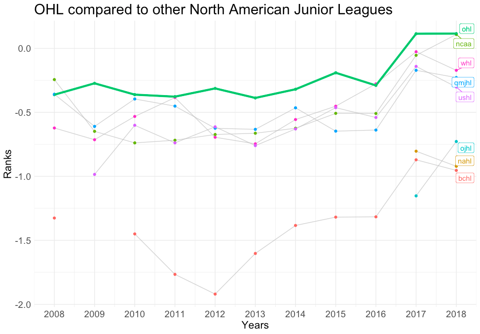
OHL versus other NA Junior Leagues: This graph displays the strength coefficients for all North American junior leagues, with the OHL highlighted in green.
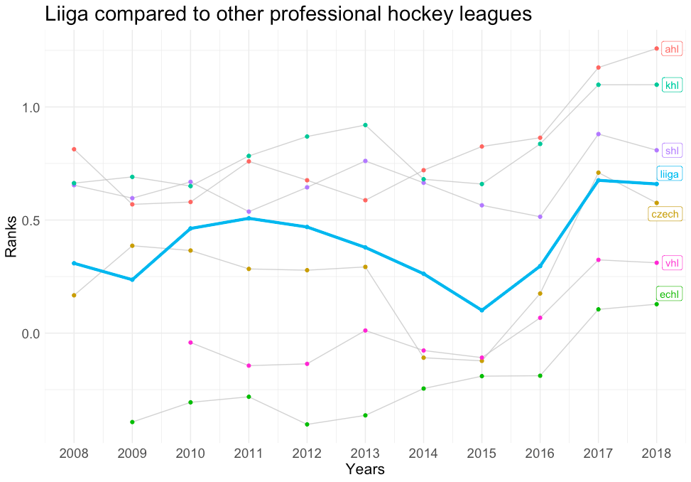
Liiga versus other professional hockey leagues: This graph displays the strength coefficients for all professional hockey leagues around the world, with the Liiga highlighted in light blue.
With the adjusted points per game player metric, not only are confounding variables such as a player’s age, position, league, and season be controlled for, which can change the outlook on the value of any given player. The modeling techniques used allow for player comparisons of hockey leagues all around the world, not just the prominent major leagues. This gives teams the ability to predict how any given player may perform in their league relative to similar players, which was previously done by using a biased estimator. The adjusted points per game metric allows for a more holistic approach for evaluating players, and provides a pathway for players that may have previously been overlooked or on the fringe. There are many applications already simply by using the adjusted points per game, but other types of data can be used as well, like scout rankings or expected goals, etc. With more detailed data in the future across all leagues, this method can also be further improved.
The research in this article was also presented at CBJHAC20 by Katerina Wu. You can find the slides here.
Follow us on Twitter @kattaqueue and @madelinejgall!

Somebody provided this thing to me off IG. But as a huge hockey fan this information is very insightful. I kind of figured the AHL would probably be the second most difficult League though.