This post assumes beginner knowledge of R.

If you’ve ever analyzed hockey data, then you’re probably familiar with the NHL’s Real Time Scoring System, which produces what’s more commonly known as play-by-play data. These data are publicly available and allow us to see every event recorded by the NHL in a given game. Shown below are selected details about the first 10 events from two games on February 18, 2019: Tampa Bay at Columbus and Vegas at Colorado.

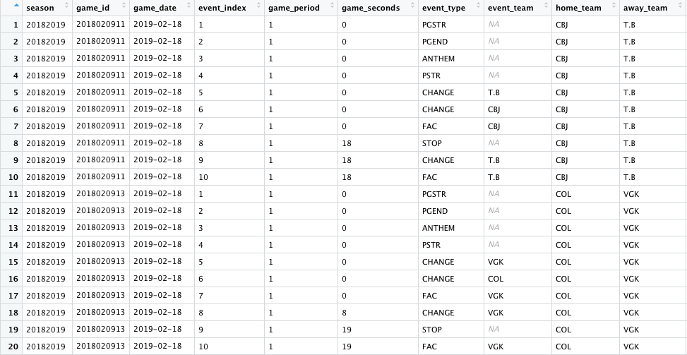
The NHL records only certain events, and there are some game seconds that have multiple events. For example, starting at row seven above, there was a faceoff to start the game, followed by 18 seconds of game play and then a stop, a change, and another faceoff.

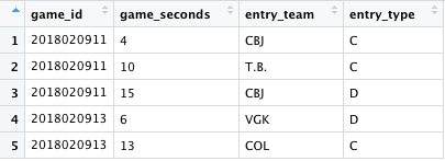
Since the NHL only records certain events, many people track games by hand in order to capture other events of interest. Most famously, Corey Sznajder tracks zone entries. Those data might look like this:

Whether you’re working with zone entry data or any other kind of manually-tracked data, you’ll probably want to join it into the play-by-play data eventually to take advantage of all the detail that’s provided by the NHL. For example, you might want to know who was on the ice during those zone entries or what the locations were for shots taken shortly after zone entries.

The obvious problem is that the game seconds (the variable we’d want to use to join the data together) don’t match up. The NHL data only contains certain game seconds: — those that indicate the time of tracked events — and those likely aren’t the same as the game seconds in your manually-tracked data. But thankfully, there’s an R package called padr that handles this problem really nicely.

The main function of padr is to adjust the desired granularity of date-time data, whether by thickening the data (aggregating it to a higher level) or padding it (inserting missing observations). And luckily for us, it works for integers, too, so we can use it for our game seconds.

The pad_int function shown above will increase the granularity of our play-by-play data so that we’ll have one row per second. The arguments to that function are, in order, the variable to be padded (game seconds), any grouping variables (the game id), and the values of the target variable where the padding should start and end. For this example, we’ll only pad the first 20 seconds. And the second function fill will, unsurprisingly, fill in certain variables.

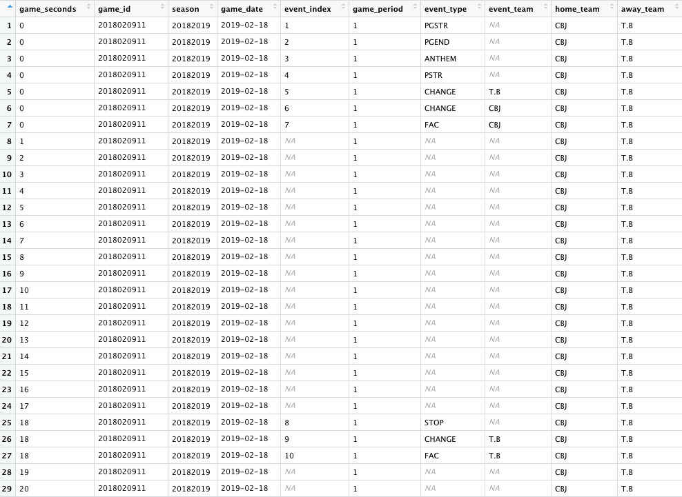
After using pad_int, that is how our data looks for one of the games. The original rows are all preserved, and there have been new observations added so that we have one row per second. We can pick out the “padded” rows since they have NA values for both the event index and the event type fields (i.e., variables that we did not include as arguments to the fill function).

Now that we have at least one observation for every game second, we can use a simple join to bring in the manually-tracked data from our previous sample data.

Now those zone entries, shown here for one of the games only, are attached to the appropriate game second and are associated with the other play-by-play data.

Variations

Different start and end values

One of the constraints of this method is that the arguments for where the padding starts and ends must be values. So what if your values aren’t consistent? For example, I often work with power play data and would only want to pad my data from the start of each power play to the end, and those values would vary within and among games. In this sample data shown below, I have a variable called PP_count that uniquely identifies each power play. I also have values for minimum and maximum seconds within the power play that identify the start and the end seconds of each power play.

We can solve this problem with a function. The code below is specific to this power play example, but the method should be adaptable to any situation in which you want to pad out your data to variable start and end values.

This function, which I called php_pad_fn, filters my data down to a single power play, saves the minimum seconds and maximum seconds as values, pads out the game seconds to and from those values, and then repeats that process for each unique power play.

Here’s a sampling of what that data will now look like:

Now we have an observation for each second on the power play and can join in other data as needed.

Multiple observations

Since we’re referencing game second here, what if you have multiple observations at the same second? If, for example, we also had a zone entry observation for game second 18 of our initial data, we’d run into a problem here because if you recall, there were three separate NHL events all recorded at that same second. If you used the code from above to join in that zone entry data, you would find this:

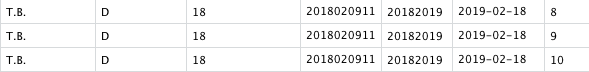
That one zone entry is now shown three times, so if you tried to sum up the number of zone entries, for example, your data would be incorrect. The ideal way to solve this problem depends a lot on your data and what kind of information you’re looking to track. But one very simple way to handle this, if you just want to match the zone entry observation to the first play-by-play observation at that second, is to do the following:

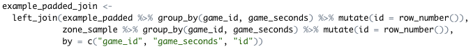
This will create a running count for each event associated with a particular game second, and you can join on that variable in addition to the game id and game seconds. That way only one zone entry observation will be added to the play-by-play data.

Hopefully the functions in this package are helpful if you want to add context to your manually-tracked data by incorporating the NHL’s play-by-play data. Data cleaning is not sexy but an essential part of the analysis process, so look for more articles on this topic coming soon from the HG team!