Relative shot metrics have been around for years. I realized this past summer, however, that I didn’t really know what differentiated them, and attempting to implement or use a metric that you don’t fully understand can be problematic. They’ve been available pretty much anywhere you could find hockey numbers forever and have often been regarded as the “best” version of whatever metric they were used for to evaluate skaters (Corsi/Fenwick/Expected Goals). So I took it upon myself to gain a better understanding of what they are and how they work. In part 1, I’ll summarize the various types of relative shot metrics and show how each is calculated. I’ll be focusing on relative to team, WOWY (with or without you), and the relative to teammate methods.

A Brief Summary

All relative shot metrics whether it be WOWY, relative to team (Rel Team), or relative to teammate (Rel TM) are essentially trying to answer the same question: how well did any given player perform relative to that player’s teammates? Let’s briefly discuss the idea behind this question and why it was asked in the first place. Corsi, and its usual form of on-ice Corsi For % (abbreviated CF%) is easily the most recognizable statistic outside of the standard NHL provided boxscore metrics. A player’s on-ice CF% accounts for all shots taken and allowed (Corsi For / (Corsi For + Corsi Against)) when that player was on the ice (if you’re unfamiliar please check out this explainer from JenLC). While this may be useful for some cursory or high-level analysis, it does not account for a player’s team or a player’s teammates.

To demonstrate what I mean, let’s revisit Joe Thornton and Jonathan Cheechoo. If you watch every goal Cheechoo scored in ’05-06 here, you may notice that Thornton is, to put it simply, doing a lot of work. While we do not have RTSS (play-by-play) data for this season, the fundamental question can still be asked: how many of these goals (or any on-ice events) were generated by Cheechoo? How many were generated by Thornton? Both Cheechoo and Thornton (and other teammate combinations with similarly high time on ice (TOI) together) will, more or less, have similar on-ice numbers whether it be goals/shots/etc. As a way to evaluate lines/combinations, on-ice numbers are often fine. But what if we want to try and separate Cheechoo from Thornton? What would that look like? How might we go about that? This is where the idea of relative shot metrics came from and why they were popularized. I’m going to mainly focus on one method here (relative to teammate), but I want to run through two other methods that are (generally) better known before we get there.

Relative to Team

Relative to Team has been written about and used for a long time, but to be honest, I actually couldn’t find where this approach first originated (or who “created” it). This metric is often referred to as “Rel” (i.e. “Corsi Rel”, “Fenwick Rel” etc.). It’s relatively simple: how did a player’s team perform when they were on the ice vs. when they were off the ice? From here on, I’m going to call this “Rel Team” to remove confusion. Additionally, I’ll be using Corsi (CF60) for each example going forward unless otherwise noted. The calculation looks like this:

Rel Team Corsi For per 60 = player on-ice CF60 – player off-ice CF60 

We often see this calculation in a differential or percentage form (Rel %, Rel Diff, etc), which takes the above “For” number and subtracts the “Against” number. This gives us a combined shots for/against number for a given player: 

Rel Team Corsi Differential per 60 minutes = (player on-ice CF60 – player off-ice CF60) – (player on-ice CA60 – player off-ice CA60)

In general, we get a better idea of how an individual player performed because we’re looking, specifically, at how a player’s team performed when they were on the ice vs. how their team performed when they were off the ice. However, this method doesn’t really address the teammate issue that is present in on-ice CF%. If a player played a large percentage of his time on a good line (or with the best teammates on his team), his respective relative to team metric will be significantly influenced by those specific teammates. And often, we’re right back to where we started. How much better was one player compared to another if they had similar on-ice and off-ice numbers? If a player plays a large percentage of their TOI with the best or worst player(s) on their team, that player’s on/off-ice numbers will be influenced in a way that makes player evaluation difficult.

With that said, this approach does have its place: it’s simple, easy to calculate, and very easy to interpret. Overall, the relative to team approach (on ice – off ice) is generally an improvement over using on-ice numbers for player evaluation as it gets closer to isolating a single player’s contribution compared to their respective team.

WOWY

WOWY (with or without you) is a slightly more complicated approach. This “metric” has also been written about in depth and is readily available on multiple hockey stats websites. The idea behind WOWY is simple: how did a given player perform WITH each teammate and how did they perform WITHOUT each teammate. This is often used alongside on-ice CF% as an addendum (Andrew Berkshire does a nice job summarizing this here, Ben Hasna covers this as well here, and David Johnson has a great in-depth explainer here).

Additionally, David Johnson’s now defunct HockeyAnalysis website provided “super WOWYs” – the ability to look not just at one player compared to each teammate but multiple players compared to multiple teammates. He sums up the standard WOWY method nicely here:

 The theory of WOWY is:

1.) if a player’s teammates generally perform better with him than apart from him that’s good,

2.) if a player’s teammates generally perform worse with him than apart from him that’s bad.

Although WOWYs can be displayed in a plain table, I find Micah Blake McCurdy’s visualizations to be one of the easiest ways to see how they work.

While WOWY’s are useful and can give us a deeper understanding of a player’s abilities based on how they performed with or without certain teammates, there are some issues with this approach. First of all, each player plays with more than one teammate, so splitting every player-teammate pair into separate observations can be misleading and can sometimes oversimplify analysis. Additionally, varying amounts of ice-time with or without a player can lead to somewhat subjective interpretations. Each player will have varying amounts of time apart from one another – where should the cutoff be? Which teammate is most important?

WOWYs are rather difficult to use outside of situational analysis. They can be great for looking at how lines are constructed, or how a given player impacted his teammates (who’s a drag, etc.), but the output is rather cumbersome – WOWYs are not meant to be “summed”. The fact that we need to look at all pairs of players at the same time introduces the possibility of misinterpretation, and comparison between players is often clumsy and difficult to set up. I love WOWYs in Micah’s visual form (above), but for any type of modeling, for instance, they’re basically useless. Ideally, we could get a single number from a WOWY… hmm, I wonder how we would do that?

Relative to Teammate – Intro

Note: it seems the method that I’m about to discuss and the “relative to team” method covered above have become, to a certain extent, synonymous based on my research. It’s important to understand that this approach is quite different from Rel Team.

The “Relative to Teammate” method was originally developed and made publicly available by David Johnson, whose HockeyAnalysis/Puckalytics websites provided the first readily available version(s). The idea behind this method is a combination of the prior two I discussed above. Relative to team gives us how a player performed relative to his aggregate team, and WOWY’s give us a big table of player-pairs that can be examined and visualized. Relative to teammate (Rel TM) combines both methods into one number. I’ve had trouble finding an article that clearly lays out exactly how this method is constructed, so I figured it would be beneficial to go through the entire calculation one step at a time. My hope here is that anyone reading this will both gain a better understanding of how the metric works, some of the issues inherent in its approach, and some of the ways we can adjust for these issues.

Let’s dive in. Here is the Rel TM calculation:

Rel TM CF60 = Player’s on-ice CF60 – weighted average of all Teammates’ on-ice CF60 without Player (weighted by Player TOI% with Teammate)

First, let’s take note of what this calculation is attempting to achieve at a high level. We see that we’re subtracting a player’s teammates’ weighted average number without a given player from that player’s on-ice number (CF60 here). So, broadly, the final number is attempting to remove what a player’s teammates did in the time they were away from that player. The theory, at least in my view, is that a player’s on-ice number is made up of what that player did plus what their “aggregate” teammates did. To find how much of a player’s on-ice CF60 can be attributed to them and how much can be attributed to their teammates, we need to find a way to measure the performance of a player’s “aggregate” teammates. This is achieved by measuring what each teammate did without that player. To determine teammate strength, we want to remove as much of the respective player’s impact as possible – hence why we are looking at teammate performance without that player. And finally, we’re weighting the “aggregate” teammate number based on the percentage a given teammate played with a given player. A player’s on-ice CF60 will consist of a higher percentage of contributions from the teammates that played the most with a given player. To account for this, the method uses a weighted average.

At the core, Rel TM revolves around the WOWY player pairs. More specifically, we need to find every teammate a given player played with during a given length of time for every player. Even early in the season – 30 games played for example – the average number of teammates all players will have played with is ~23 (excluding players who changed teams), and ~750 players will have played > 0 minutes. To calculate Rel TM at the 30 game mark, we’re looking at ~18,000 pairs of players. 

The Calculation

Disclaimer: all of the numbers I’ll be using are from the NHL’s play-by-play data. The data was scraped using Emmanuel Perry’s (Manny’s) NHL Dryscrape functions, and I wrangled/organized/cleaned the data myself. Because of this, there may be a few differences between my data and other publicly available data (broken games, etc.). I will be making my R code, final season-by-season numbers, and WOWY tables available at the end of part 2.

We can use any metric we like with this approach (Corsi, xG, SOG, hits probably, why not?). Just like the Rel Team method, we can also look at both for and against numbers individually. For the purpose of this article I’ll be sticking to even-strength situations, but this can be applied to any strength state.

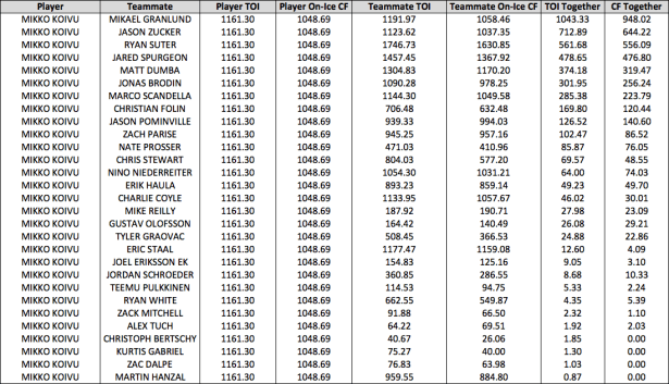
To demonstrate, I’m going to use Mikko Koivu’s ’16-17 season to explain how Rel TM is calculated (I’ll be using CF60 in this case). First we collect the following: Koivu’s total TOI and raw on-ice CF, each of Koivu’s teammate’s total TOI and raw on-ice CF, and Koivu’s TOI and raw on-ice CF with each teammate. That looks like this:

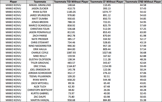
Next, we determine each of Koivu’s teammate’s TOI and CF without Koivu (each teammate’s TOI and CF minus the TOI and CF they spent with Koivu) and convert this number to a per 60 minute rate:

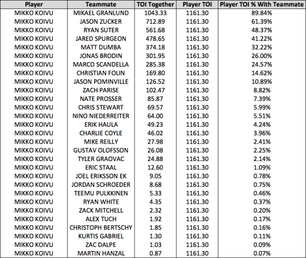
We then calculate the percentage of Koivu’s TOI that he spent with each teammate (used for the weighted average). For instance, Koivu played 1161.30 EV minutes total. He played 1043.33 EV minutes with Mikael Granlund. His TOI% with Granlund is 1043.33/1161.30 = 89.84%. This is done for each of Koivu’s teammates:

With the numbers above, we can calculate the weighted average. A quick note: I’ve displayed the percentage for ease of viewing, but we use the decimal version (.8984 for instance) for every step in the calculation.

Each of Koivu’s teammate’s CF60 without Koivu is multiplied by the “Player TOI % With Teammate” number that we just calculated:

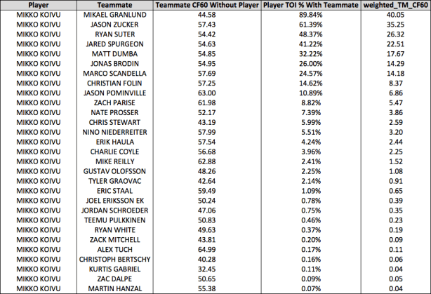
We then sum the “weighted TM CF60” numbers and divide by the sum of the “Player TOI % With Teammate” number – if 5v5 is used this will sum to 4 (the number of teammates during this strength state). If EV is used it will vary slightly (4v4 and 3v3 impact this number a bit). Over 10 years, the average number of teammates a player had during EV play was 3.978 (for reference). In this case, the sum of the “weighted TM CF60” column is 211.01, the sum of the “Player TOI % With Teammate” column is 3.96. We divide the first by the second (211.01 / 3.96) to arrive at 53.27. This is the weighted average of Koivu’s teammates’ CF60 without Koivu.

We now have the “right side” of the calculation I laid out at the beginning of this section (weighted average of all Teammate on-ice CF60 without Player [weighted by Player TOI% with Teammate]). The “left side” is the player’s on-ice CF60. The final calculation is:

Koivu’s Rel TM CF60 = 54.18 – 53.27 = .91 

To calculate his Rel TM Corsi differential (Koivu’s Rel TM CA60 in ’16-17 was -3.84), we take Rel TM CF60 – Rel TM CA60 (.91 – (-3.84)), which equals 4.75. With this number, we can say that Koivu netted 4.75 shot attempts per 60 minutes relative to his teammates by this metric (about 70^th percentile in ’16-17). For reference, the highest Rel TM Corsi differential per 60 among forwards (minimum 500 even strength minutes) for the ‘16-17 season was Artemi Panarin’s 22.74 (9.87 Rel TM CF60 and -12.87 Rel TM CA60), and the lowest was Chris Stewart’s -20.12 (-13.29 Rel TM CF60 and 6.83 Rel TM CA60).

Relative to teammate numbers are often shown as a percentage above/below 0 as well. This is done after both the weighted average of a player’s teammates’ without numbers “for” and “against” have been calculated. It looks like this:

Rel TM CF% = (on-ice CF60 / (on-ice CF60 + on-ice CA60)) – (weighted teammate CF60 / (weighted teammate CF60 + weighted teammate CA60)) 

Problems

In an abstract sense, all relative to teammate methods inevitably suffer from “multicollinearity” when players spend a large amount of time together. This has been noted in various ways by Manny here, Brian MacDonald here, Shane Jensen here and here, A.C. Thomas et al. here, and Dawson Sprigings here among others.

Manny quite succinctly dubbed this the “Sedin Paradox”. With a large enough sample, the multicollinearity issue isn’t as problematic; however, in small samples and with player-pairs like the Sedins, this can be a huge problem. Even during a full season, pairs of players often play so much time together (90%+) that their relative numbers will be heavily influenced by what one teammate did in a relatively small number of minutes away from that player. This problem becomes apparent with the way the weighted average is calculated (a player’s teammates who played the most with that player are given the most weight in the calculation).

To demonstrate how early season/small sample issues can be problematic, let’s look at Ryan Suter and Jared Spurgeon through 16 games of the ’17-18 season. Spurgeon had only played 12 minutes away from Suter at even-strength, and Suter had played 90% of his EV TOI with Spurgeon. Spurgeon’s total on-ice CF60 at that time was 58.8, however, in the 12 minutes he played away from Suter his CF60 was 74.1. So, ~25% of Suter’s weighted teammate CF60 without was the 12 minutes of CF60 Spurgeon spent away from Suter.

We see the same thing over the course of an entire season if a pair of players play enough time together (hence the Sedin paradox). In the ’08-09 season, Daniel and Henrik played 1130 and 1150 total minutes respectively (I’m rounding a bit here). Of those minutes, 1060 minutes were spent together (Daniel spent 90 minutes apart from Henrik and Henrik 70 minutes apart from Daniel). So ~25% of Daniel’s weighted teammate component will be based on the 70 minutes Henrik played without him. This is a problem.

Adjustments 

To adjust for the above issue, David Johnson’s original Rel TM calculation didn’t split into a teammate’s “without” number until that player had played more than 100 minutes away from any given player. Using the Sedin example, neither brother’s CF60 without would have factored into their respective brother’s Rel TM number for that season. Instead, each Sedins’ without number would be replaced with their respective on-ice number. Manny proposed an approach to this problem that used a bootstrap resampling method to adjust for when a player’s TOI % with a teammate exceeded 3 standard deviations from the mean. Due to the marginal gains and computational costs of this method, he elected to forgo this approach.

This is an issue that I feel should be accounted for, and I wanted to keep this all “pen and paper” so-to-speak, so I’ve used Johnson’s original approach as a starting point. While Johnson’s method makes a lot of sense, I felt instead of completely eliminating certain player-pairs from the calculation, it might make more sense to blend a player’s on-ice number with their teammates’ without number when a teammate has not played sufficient time away from a player. So… where should we set the TOI cutoff? Is Johnson’s 100 minutes mark correct? A simple way to determine this is to look at CF60/CA60 without player plotted against EV TOI without player to try and determine where CF60/CA60 stabilizes. Here are all forwards and defensemen over the last 10 years:

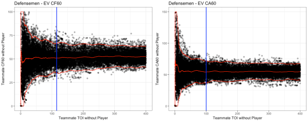
Using Dawson Sprigings’ method linked in the slides here, I added lines that show 2 standard deviations from the mean above and below average. After testing using ten years of data, individual seasons, and limiting this to the first 20, 30, and 40 games of every season, it appears that CF60 stabilizes at ~90 minutes for forwards and ~115 minutes for defensemen (for CA60 it’s ~125 minutes for forwards and ~100 minutes for defensemen). I will use this for the threshold under which the teammates’ numbers need to be blended. Additionally, these rates do not stabilize linearly, so I’ll use an “exponential” method to estimate this effect. The blending looks like this:

Forward adjusted wTM_CF60  =  wTM_CF60 * (TOI_w.o^2 / 90^2) + CF60 * (1 – (TOI_w.o^2 / 90^2))

Defensemen adjusted wTM_CF60  =  wTM_CF60 * (TOI_w.o^2 / 115^2) + CF60 * (1 – (TOI_w.o^2 / 115^2))

To demonstrate, I’ll stick with the Suter/Spurgeon example from earlier and look at the “right side” of the calculation for Suter’s Rel TM final number. Instead of using all of Spurgeon’s CF60 w/o Suter for the weighted average, we will substitute the following:

74.1 * (12^2 / 115^2) + 58.8 * (1 – (12^2 / 115^2)) = 59.0

Let’s pretend Spurgeon had more TOI away from Suter just for demonstration – let’s say 80 minutes:

74.1 * (80^2 / 115^2) + 58.8 * (1 – (80^2 / 115^2)) = 66.2

Spurgeon’s CF60 without Suter is very close to his total on-ice CF60 in the first calculation since he’s only played 12 minutes away from Suter. As he plays more TOI without Suter, this will move closer to the full CF60 without Suter.

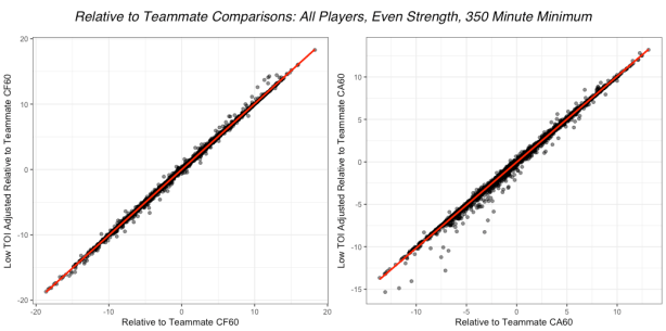
This calculation is carried out for each of Suter’s teammates and substituted for the CF60 without figure when a teammate’s TOI apart from a player is less than 90 min for Forwards or 115 min Defensemen. This will be done for almost all players at the beginning of the season, but after a full season this adjustment only impacts a select few players – specifically the Sedins and player-pairs like them. Below is a plot comparing the “unadjusted” and “low TOI adjusted” methods for reference (I’ve included CF60 and CA60 and included only qualified players):

Team Effects

Additionally, I have found that team strength has an impact on the final Rel TM number. After adjusting for the low TOI % player-pairs, there still appears to be a team-strength bias. Specifically, players on the worst teams appear better and players on the best teams appear worse relative to the league. This effect can be demonstrated by looking at qualified players who changed teams from one year to the next. If we plot the change in each player’s weighted average of teammate without player metric (the “right side” of the Rel TM calculation) against the change in the respective Rel TM metric from “year 1” to “year 2”, we can see this relationship:

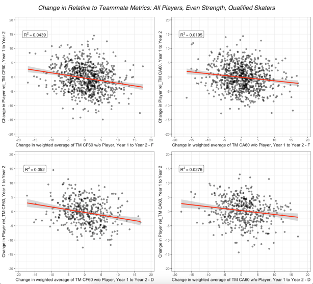
From year 1 to year 2, there is a slight relationship between the change in a player’s strength of teammates (weighted average of TM CF60/CA60 without) and the change in that player’s respective rel TM CF60/CA60. If the team a player played on did not influence a player’s Rel TM metric, we’d expect to see no relationship between these two metrics. The fact that a negative trend is observed indicates that team effects are present.

This is a rather tricky issue to address. My thought here is that there are “bounds” for on-ice CF60/CA60 and weighted TM CF60/CA60 and they are not equal – for instance, it is possible that there is an upper-limit to on-ice CF60 that is not present (or equal) to the weighted teammate average counterpart. My solution to adjust for this is to “shrink” each player’s weighted TM metric to league average (per season). I centered and “regressed” the weighted teammate without metric until the above plot/relationship returned an R-squared value of ~0. The exact amount of “shrinkage” was determined by testing on multiple player season TOI cutoffs for both CF60 and CA60. It was determined that the amount of shrinkage for weighted TM CF60 was .81 and for weighted TM CA60 was .88 – I found that player position (F/D) had no effect on these numbers. The calculation for this adjustment looks like this:

Adj. weighted TM CF60 = ((weighted TM CF60 – NHL average weighted TM CF60) * .81) + NHL average weighted TM CF60

Adj. weighted TM CA60 = ((weighted TM CA60 – NHL average weighted TM CA60) * .88) + NHL average weighted TM CA60

We can plot the prior chart again and see the adjustment:

It is important to note that this is an estimated team-effect adjustment. It has been added to more accurately compare players across teams. Overall, I feel both the low TOI % adjustment and the team effect adjustment do a very good job dealing with the innate problems the Rel TM method poses. In part 2, I’ll explore the relationship between Rel Team and Rel TM, dig into the WOWY tables to further explore how the Rel TM calculation works, and analyze the team adjustment I’ve presented here in greater detail.