In part 1, I described three “pen and paper” methods for evaluating players based on performance relative to their teammates. As I mentioned, there is some confusion around what differentiates the relative to team (Rel Team) and relative to teammate (Rel TM) methods (it also doesn’t help that we’re dealing with two metrics that have the same name save four letters). I thought it would be worthwhile to compare them in various ways. The following comparisons will help us explore how each one works, what each tells us, and how we can use them (or which we should use). Additionally, I’ll attempt to tie it all together as we look into some of the adjustments I covered at the end of part 1.

A quick note: WOWY is a unique approach, which limits it’s comparative potential in this regard. As a result, I won’t be evaluating/comparing the WOWY method further. However, we’ll dive into some WOWYs to explore the Rel TM metric a bit later.

Rel Team vs. Rel TM

Note: For the rest of the article, the “low TOI” adjustment will be included in the Rel TM calculation. Additionally, “unadjusted” and “adjusted” will indicate if the team adjustment is implemented. All data used from here on is from the past ten seasons (’07-08 through ’16-17), is even-strength, and includes only qualified skaters (minimum of 336 minutes for Forwards and 429 minutes for Defensemen per season as estimated by the top 390 F and 210 D per season over this timeframe).

Below, I plotted Rel Team against both the adjusted and unadjusted Rel TM numbers. I have shaded the points based on each skater’s team’s EV Corsi differential in the games that skater played in:

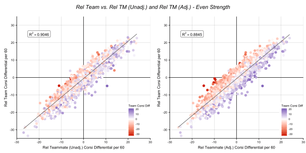Initially, we can see that Rel Team and Rel TM are, visually, quite similar, and the R-squared values for both show this as well (Pearson R of .9511 for unadjusted and .9405 for the adjusted). Notice that the R-squared value is slightly higher for unadjusted Rel TM compared to adjusted Rel TM, the team Corsi differential shading is a little more random for the unadjusted version, and there is a more pronounced red to blue fade in the adjusted Rel TM chart. This “fade” shows us one of the biggest differences between the two metrics: Rel TM (adjusted more than unadjusted) appears to “penalize” players on “bad” teams and boost players on “good” teams when compared to Rel Team. We also see this when we compare the unadjusted and adjusted versions of Rel TM:

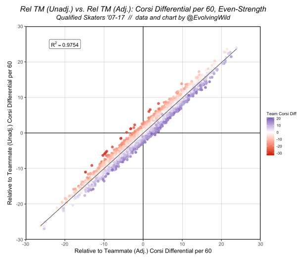
There is a perfect split along the line of best fit. The team adjustment is clearly altering the overall values of the unadjusted Rel TM metric – even if it is somewhat minimal. With the three plots shown, we see a distinct difference between the adjusted and unadjusted versions of Rel TM. Additionally, the correlation between unadjusted Rel TM and Rel Team is higher. To explore these relationships further, I think isolating players with significantly different Rel Team and Rel TM numbers may give us a bit more information about what’s going on here.

Outliers

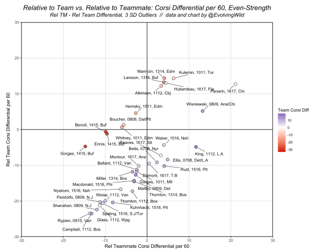
There are a few players who see a +/- 10 Corsi differential per 60 change from Rel Team to Rel TM, and there are plenty of players who move from “positive” to “negative” impact players. Here, I’ve isolated the qualified skaters with the biggest difference between Rel Team and Rel TM Corsi differential per 60 in a single season over the past 10 years (more than 3 standard deviations from the mean):

And here are the two biggest positive and negative changes among skaters from the above chart:

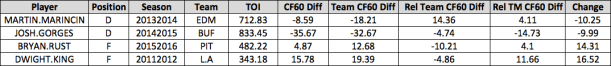
On the very edge, we see the team impact quite clearly. Gorges and Marincin played on terrible teams and their on-ice differentials reflect this. Rust and King played on very good team and their on-ice differentials reflect this as well. Rel Team, however, almost entirely reverses this, which kind of makes sense. Relative to Team essentially treats every team as “0” – it doesn’t care how good or bad any given team is, every player is evaluated relative to the team, and all teams are equal. It doesn’t matter if it’s Buffalo in ’14-15 or LA in’11-12, both of these teams are the “same” from a Rel Team perspective. This raises some concerns.

If we plot Rel Team, unadjusted Rel TM, and adjusted Rel TM against Team Corsi in the games each player played in (differential per 60 for everything), we see an interesting relationship:

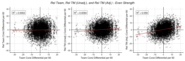
Team Corsi differential accounts for basically none of the variance in Rel Team Corsi differential (.0002), unadjusted Rel TM is similar in that regard, and adjusted Rel TM Corsi differential shows a slight increase. Granted, this is still a very small explanation of the variance, but for our purpose, it more or less confirms how Rel Team and unadjusted Rel TM deal with team effects: they remove them entirely. Buffalo and LA are the same team, and the players on those teams are treated the same. The team adjustment for Rel TM appears to “add back” some aspects of team strength.

Note: For simplicity’s sake, I will be using the team-adjusted version of Rel TM going forward (unless otherwise noted).

Because the “left side” of each metric is on-ice Corsi, let’s take a look at Rel Team and Rel TM in comparison to the respective on-ice Corsi differential (again, shaded by the same team Corsi differential per 60 used above):

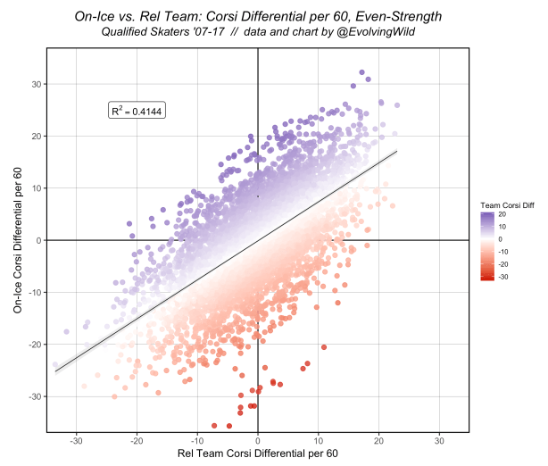
You’ll notice there is a perfect color gradient in the Rel Team chart, where Rel TM is bit less perfect – we’re seeing the simplicity of Rel Team here as there is no weighting or adjustment. The R-squared value is also much lower with Rel Team, which me might expect given the literal 0 correlation from above. So, we now see that Rel Team removes all team effects in its output. That may actually seem beneficial at first, but if we look at how on-ice Corsi differential compares to Team Corsi differential, we see a potential problem: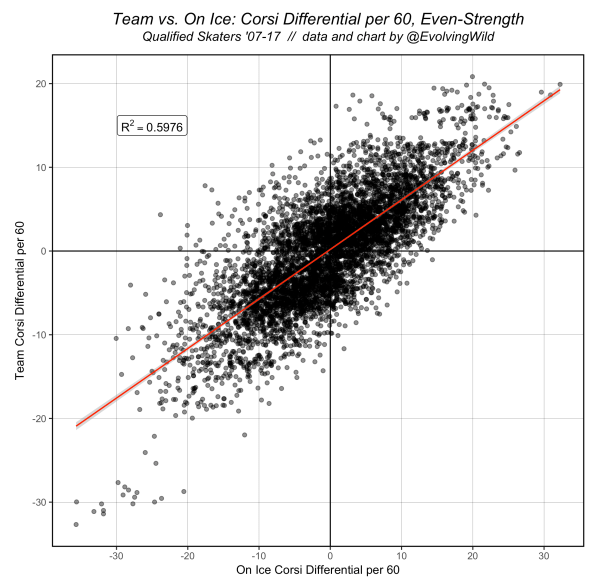

For our purpose, what matters here is that the R-squared value we see is much higher than the Rel Team ~ On-ice R-squared value in the earlier chart. Rel Team appears to be removing a lot of the team influence, but is that correct? It’s a chicken-and-the-egg scenario: is player X’s team good because of player X? –OR– is player X good because player X’s team is good? I’m not really sure we can answer that (right now), but it’s important to acknowledge this. With the Rel TM comparison, we actually see an R-squared value that is very close to the above chart (.0088 higher than Team ~ On-ice to be exact). For me, that’s a good indication that we’ve reached something that adjusts for team effects appropriately. While I think there is more that could be explored in the above chart, let’s leave that for another time and move on.

Panarin / WOWY analysis

I wanted to dive into a situation that’s a bit rarer – I’ll just call it the “Panarin situation” because I love Panarin (of note: this happens quite often to a much smaller degree). There were only two players in the outlier chart referenced earlier who had positive Rel Team numbers and saw a marked increase in Rel TM (when compared to Rel Team). Here they are:

I’m going to leave Wisniewski out of this for now (he played for two teams, his TOI was much lower, etc). The Chicago Blackhawks in ’16-17 were by no means special as a team when Panarin was in the lineup per his Team Corsi differential – they were actually only slightly above the prior 10-year average. Additionally, his Rel Team metric is about 1.5 standard deviations above the mean, which is a decent increase from his on-ice CF60 differential, but nothing incredible. So what’s going on here? This example is a good time to dive further into how Rel TM measures players – for that we need to go back to the WOWY tables:

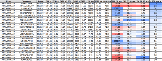
Panarin played on a line with Patrick Kane and Artem Anisimov for the majority of the ’16-17 season, (as the “p_TOI_perc_w” – player TOI % with – column shows). But we see something else: Kane and Anisimov were not good without Panarin, especially Kane – he played 400+ minutes away from Panarin in ’16-17 (which by itself would be a “qualified” season). The Rel TM calculation weights a given metric based on this TOI%, remember, and Kane and Anisimov make up almost 35% of the weighted teammate portion of Panarin’s overall Rel TM calculation. Panarin’s on-ice Corsi differential per 60 was 10.47 (the “left side” of the equation), an incredible amount higher than Kane and Anisimov’s without numbers. Rel TM is telling us that Panarin drove this line, and Kane and Anismov benefitted from playing with Panarin.

As I’ve mentioned above, there are still some potential issues that we should explore. For instance, Anismov only played ~130 minutes away from Panarin. Some may take exception to the fact that ~15% of the total weighted average of Panarin’s teammates’ number is based on Anisimov’s play away from him, but I’d argue that this makes sense. 85% of this weighted average is made up of each other teammate, and you might expect another teammate to even this out somewhere else (Kempny in this case). There are some unusual situations of course, but I’ve found that by and large, the number of players impacted incorrectly after adjusting for both early-season/high % pairs and team effects is marginal.

WOWY Example #2

Let’s look at another WOWY that’s not quite as clear (but still comes from one of our outliers above). Here is Matt Marincin from the ’13-14 season:

Remember, Marincin was on the other end of the spectrum here – his Rel TM Corsi differential per 60 decreased by ~10 in comparison to his Rel Team Corsi differential per 60 (14.36 to 4.11). Also remember the ’13-14 Edmonton team was terrible (the Oilers’ Corsi differential per 60 was -18.21 in the games Marincin played in), and his on-ice Corsi differential per 60 was -8.59, which was well above the team’s differential.

Here we see that the five highest TOI% players were all better when playing with Marincin than they were when playing without him. At the same time, Marincin wasn’t nearly as good as Rel Team would have you believe (due to the stark nature of just how bad this Edmonton team was). His unadjusted Rel TM Corsi differential per 60 here is 6.22, but after adjusting for team strength (the team adjustment is applied after the weighted average), we see his final adjusted Rel TM Corsi differential per 60 drop to 4.11. We’ve already seen how much better a player on a team like the ’13-14 Edmonton Oilers can look from a relative approach without accounting for team strength, so this fairly significant adjustment makes sense. Overall, Marincin was good with Edmonton this season, but taking his teammates and the strength of his team into his account, we see that the Rel Team method overvalues him.

I’ve been referring to the top 5 teammates here, which was intentional: from ’07-17, a given player’s top 5 or 6 teammates based on TOI%-with account for ~50% of a given player’s weighted without number in the calculation (for Marincin, the top five players make up 51.34%). This, I think, is one of the more important things to understand with this method, especially if you plan on digging into the WOWY numbers to figure out why a player looks the way they do. Proportionally, a teammate who’s played <10% with a given player, for instance, has very little impact on that player’s Rel TM number. The top 10 teammates account for ~75% of the weighted teammate portion of the metric, and the top 15 teammates account for ~90%.

Team Adjustment – Part 2

With all of this in mind, let’s take a look at the team adjustment a bit more. Here’s a chart showing how the team adjustment differential compares to every player’s team Corsi differential (both per 60):

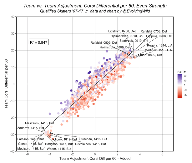
I’ve labeled the players with the biggest negative (bottom left) and biggest positive (upper right) team adjustments. The Rel TM coloring isn’t as important for the biggest team adjustment players; we’re more concerned with which players see the largest impact from the team adjustment. Here’s a table where I’ve isolated three groups of players based on their individual team adjustment (highest, lowest, and “no adjustment”):

The players who see the largest adjustment play on teams that are either very good or very bad. The team adjustment is attempting to correct for the over/undervaluation of players that results from both the Rel Team and Rel TM methods’ innate “zeroing” effect on team strength. Additionally, if we look specifically at individual teams, we can see how the team adjustment impacts all players on a single team. Here I’ve isolated the ’13-14 Oilers, the ’10-11 Predators, and the ’11-12 Kings to give us “good”, “average” and “bad” teams:

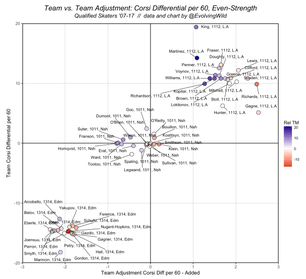
We see that each team centers around the team mean and no player moves +/- 1 point within the team mean. Additionally, we see that “good” players (darker blue shading) see a reduction and “bad” players see a boost (within their respective teams). If you pop back up to the “Team vs. Team Adjustment” chart, you can see this in the Rel TM shading as well. This trend is the result of the team adjustment attempting to correct for the “zeroing” effect previously discussed. What’s interesting is that while the adjusted Rel TM approach “penalizes” the entire team, within each team it’s the worst players who are effected the least (on average).

The overall effect comes back to the way the team adjustment calculation works. Let’s refresh our memory:

Adj. weighted TM CF60 = ((weighted TM CF60 – NHL avg. weighted TM CF60) * .80) + NHL avg. weighted TM CF60

Adj. weighted TM CA60 = ((weighted TM CA60 – NHL avg. weighted TM CA60) * .88) + NHL avg. weighted TM CA60

Remember, this is only applied to the “right side” of the Rel TM calculation – the weighted teammates portion – this more or less “regresses” every teammate towards the league mean. So while any given player’s on-ice number (the “left side”) will stay the same, the weighted teammates number is brought closer to league average. This is what we see above: the “best” players, regardless of their team, will see a larger negative adjustment on average because their teammates’ numbers (who were always worse without them) will move closer to league average (these teammates get better). The same thing happens with the “worst” players – their “better” teammates move closer to league average as well. In the final calculation, a “good” player’s teammates improve when compared to the Rel TM calculation without this adjustment, and vice versa.

Overall, the team adjustment allows us to more accurately evaluate players on different teams. As we’ve seen, the Rel Team and unadjusted Rel TM method remove all team effects, which means that any comparison of two players on different teams assumes those teams are equal. This is incorrect. Teams vary in strength. If we’re looking to evaluate players across the league, we need to look not at how each player performed relative to their team but how a player performed relative to their team relative to the league.

Evaluating Team Strength

Finally, let’s see what these metrics look like when compared to team totals. One of the biggest issues with the relative metrics, as I’ve (hopefully) shown, is that the sum of a team’s parts (each player) does not equal the actual team sum. To demonstrate, I took every team over the prior 10 seasons (’12-13 season excluded), found their total even-strength Corsi differential, and summed each player’s relative “impact” when on the team. This “impact” calculation is the “expanded rate” that results from the respective relative method. The calculation looks like this:

Rel TM Corsi Impact = (Rel TM Corsi diff60 / 60) * TOI

This gives us a “raw” differential that can be summed for each player on each team. For this comparison, I have separated out players who were traded, so their contribution to each team (within each season) is included in the “player summed” total.

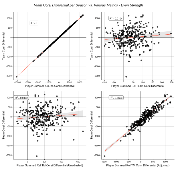
The total of each team’s players’ on-ice Corsi differentials sum perfectly to the respective team Corsi differential multiplied by five (the total number of on-ice skaters). Rel Team and unadjusted Rel TM remove almost all team effects, so the .01 R-squared value isn’t that surprising. However, after adding the team adjustment to the Rel TM method, we see that the team effects have been added back. While the player-summed Rel TM figures do not sum perfectly to the actual team Corsi differential, we’re now much closer. I find it important to note that while the aggregate on-ice and the adjusted Rel TM Corsi differentials have very high R-squared values (for on-ice it’s perfect), on-ice and Rel TM Corsi differential when compared to one another have an R-squared value of .61 (from the chart in part 1). So while they explain a team’s Corsi differential similarly, they are still different.

Taking this a step further using the same data, I substituted team goal differential (all situations excluding shootouts) and compared the same four metrics:

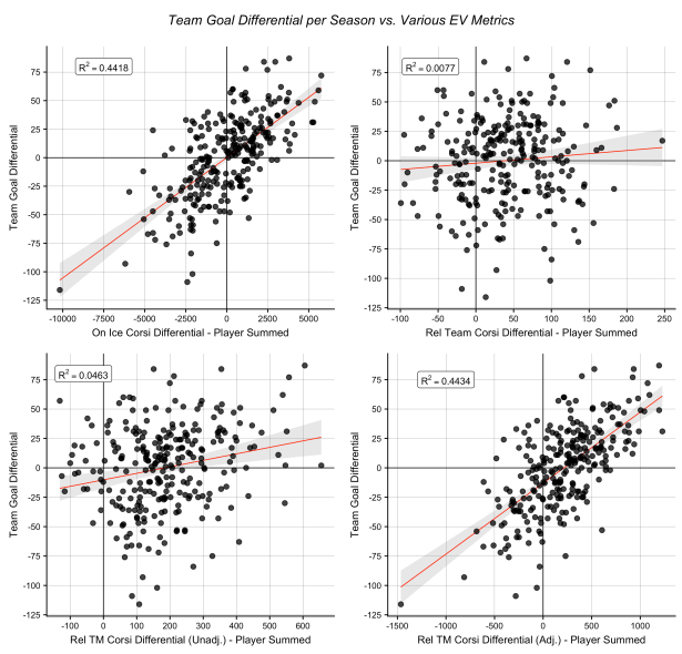
Here we see similar results, but the R-squared values decrease. Rel Team and unadjusted Rel TM still do a very poor job of describing “team strength”, while on-ice and adjusted Rel TM are much better. Adjusted Rel TM is slightly better here but they’re close enough that I’d consider them basically the same. Regardless, this supports the overall point: adjusting the Rel TM method to account for team strength allows the Rel TM method to better explain the team strength we’re adjusting for to begin with. Additionally, this allows for player comparison from one team to another.

Conclusion

There are a few points that I hope can be taken away from all of this. The first being: relative to team and relative to teammate are not the same thing; these methods evaluate players in very different ways. Additionally, for every type of long-term player evaluation, I feel the adjusted Rel TM method is vastly superior to the Rel Team method. There are a few situations, however, where I feel it may be beneficial to use Rel Team:

1. You would like to see how a given player has performed in a small sample (< 15 games – in my opinion, you’re probably better off waiting until there is more data)
2. You would like to actually evaluate how well a player performed relative to his team. In this situation it’s assumed you only care specifically about one team.
3. You would like to evaluate how a player performed in one game. This is similar to point 1, but in small samples, the Rel TM method is basically unusable.
4. You don’t have access to a relative to teammate metric.

In my opinion the relative to team method is mostly useless outside of the above situations. In small samples for player evaluation it’s not entirely useless, but I think in general you’re better off waiting until more data is available. Relative to teammate allows us to convert a player’s WOWY into a single number that is more useful for player evaluation. After adjusting for the low time-on-ice and team strength issues, we see that the sum of all player contributions for each team now equal (more or less) that team’s strength. This allows us to compare players across teams in a way that both the Rel Team and unadjusted Rel TM methods do not. In general, I feel the Rel TM method – when adjusted for its inherent issues – is one of the best single-number “pen and paper” methods we have at our disposal for player evaluation.

 

Acknowledgements

I would like to thank the following individuals:

• David Johnson for his work creating and developing the Rel TM method
• Matt Cane and Dawson Sprigings for their assistance with the calculation
• Emmanuel Perry for his NHL play-by-play scraper available on his GitHub page

Data

• The R code for the Rel TM method is available on my GitHub here:
• The season-by-season Rel TM data (adjusted for team and unadjusted for team/TOI) is available in a google doc here. Unfortunately, the 10-season WOWY data is too large to host on my GitHub page (250,000+ rows). If you would like this data, I can be reached @EvolvingWild on Twitter. Feel free to reach out.