
This piece is co-authored between DTMAboutHeart and asmean.
Introduction
Expected goals models have been developed in a number of sports to better predict future performance. For sports like hockey and soccer where goals are inherently random and scarce, expected goals models proved to be particularly useful at predicting future scoring. This is because they take into account shot attempts, which are better predictors of a team and player’s performance than goal totals alone.
A notable example is Brian Macdonald’s expected goals model dating back to 2012, which used shot differentials (Corsi, Fenwick) and other variables like faceoffs, zone starts and hits. Important developments have been made since then in regards to the predictive value of those variables, particularly those pertaining to shot quality.
Shot quality has been the subject of spirited debate despite evidence suggesting that it plays an important role in predicting goals. The evidence shows that shot characteristics like distance and angle can significantly influence the probability of a certain shot resulting in a goal. Previous attempts to account for shot quality in an expected goals model format have been conducted by Alan Ryder, see here and here.
In Part I, an updated expected goals (xG) model will be presented that accounts for shot quality and a number of other variables. Part II will deal with testing the performance of xG against previous models like score-adjusted Corsi and goals percentage.
Part I
All data is from even-strength situations
In addition to using Fenwick shots, the regression model accounted for several variables** that have an effect on the likelihood of a shot ending up in a goal: 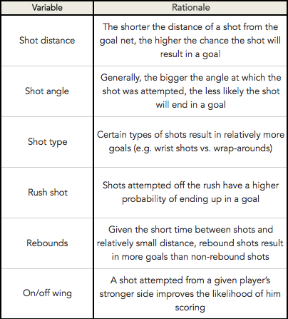
The model also takes into consideration shooter talent, which we know varies significantly from player to player. Accounting for shooting talent makes intuitive sense, as we expect that shots attempted by Brad Marchand on average have a higher likelihood of resulting in goals than shots taken by, say, Tanner Glass. To this end, a “Shot Multiplier”*** was developed to approximate a player’s effect on each shot’s probability of resulting in a goal. The Shot Multiplier was determined by following these steps:
- Regressed Shots: the number of shots for which 5-on-5 Sh% for forwards and defensemen begins to stabilize was determined using Kuder-Richardson Formula 21 (K-R 21). Sh% stabilized at approximately 375 shots for forwards and 275 shots for defensemen. For each forward, 375 shots were added to the player’s season shot total. Similarly, 275 shots were added for each defenseman’s total season shots. For explanation purposes this number of added shots will be designated as regressed shots, or rShots.
- Regressed Goals: a player’s regressed goals (rGoals) was calculated by multiplying a player’s season goal total by (rShots * league average Sh%). Note: rShots is 375 or 275 depending on if the player is a forward or defenseman, respectively. Similarly, forwards and defensemen had different league average Sh%.
- Regressed Sh%: was calculated by dividing a player’s rGoals by rShots.
- Shot Multiplier: was computed by dividing a player’s regressed Sh% (rSh%) by the league average Sh%.
Finally, each player’s shot was multiplied by their Shot Multiplier. Steps 1) to 4) can be followed along the table below, which uses Steven Stamkos’ 2011-2012 season as an example:

Part II
Data from the 2012-13 lockout-shortened season was excluded
To test how this expected model performs against previous models like score-adjusted Corsi and goals %, year-to-year correlations were performed using the methods described by Jlikens here, with some changes. The first test consists of an in/out sample to determine how past results predict future results at the team level. Given the relative complexity of the test, the methods will be detailed below in a stepwise fashion:
- Select a random sample of X number of games in a season, which will make up Group A. Group B will be the remaining number of games in the season
- Choose a metric of interest (e.g. CF%) and calculate it for Groups A and B
- Calculate the correlation between Group A and Group B for each Team-Season (using 30 teams * 7 seasons = 210 Team-Seasons)
- Repeat steps 1) to 3) 1000 times
- Using Fisher-Z transformation, convert all correlations obtained into Z
- Convert Z into an R value
- Repeat steps 1) to 6) for every 10-game interval (10, 20, 30, …, 70)
- Repeat steps 1) to 7) for each metric
It should be noted that step 4) was repeated 1000 times to smooth out any correlation quirks that can arise when working with random samples. In step 7), intervals of 10 games were chosen arbitrarily to save time, as the number of games in an interval has no significant bearing on the final conclusions reached by the model.
The second test performed is a modified version of Emmanuel Perry’s previous work found here. This test determined how past results predict end of season statistics (or final results). It follows the same steps as the first test, except that Group B consists of end of year statistics.
The same tests were carried out at the player level. The analysis was restricted to players who dressed for at least 80 games in a given season. The resulting sample consisted of approximately 1000 player-seasons. Given the large sample of player-games, step 5) was only repeated 25 times for on-ice stats and 100 times for shooting stats.
Finally, root mean squared error (RMSE) values were computed for each statistic.
Results
- Expected Goals at the Team Level
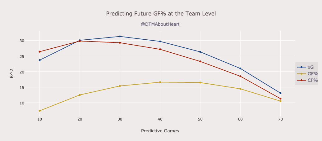
At the team level, xG has the same predictive power at the 20-game mark as score-adjusted Corsi (CF%) and Goals For (GF%) but proves to be a far more superior predictor of future goals past that mark (Figure 1). Note that xG also outperformed CF% and GF% with regards to root mean squared errors (RMSE).
Figure 1

Table 1

Table 2
- Expected Goals at the Player Level
xG also predicts future goals better than (score-adjusted) CF% and GF% at the player level. A comparison of Figures 1 and 2 shows that xG’s higher correlations can be appreciated sooner than for xG at the team-level. As early as the 10-game mark, xG outperforms previous models:

Figure 2

Table 3

Table 4
- Expected goals and individual performance
xG also better estimates future individual scoring. As seen in Figures 3-4 and Tables 5-6 below, individual xG per 60 minutes (ixG/60) outperforms iCF% and Sh% across the board:

Figure 3

Figure 4

Table 5

Table 6
As described above, xG is significantly more predictive of future goal scoring compared to previous models. In addition to being predictive, xG also appears to have superior descriptive power as it explains more of the variance in GF% than score-adjusted Corsi at the team level. Note that removing the two Buffalo outliers from the data presented in Figures 4 and 5 below did not significantly affect the correlation values.

Figure 5
Conclusion and Future Directions
Expected Goals (xG) significantly outperforms score-adjusted Corsi (CF%) and Goals For (GF%) in predicting future goals at the team and player levels. xG is also descriptive, which makes it a superior tool in evaluating a team and player’s past and current offensive performance. All data is posted in the spreadsheet below.
An obvious future direction would be splitting forwards and defensemen for analysis at the player level. Presumably, variables included in this xG model can vary in their descriptive and predictive value when testing for defensemen and forwards separately.
Lastly, future work will also include looking at special teams, as one would expect that the significance of predictor variables would differ from even-strength situations.
Acknowledgments
Thanks to Austin Clemens for his graphics code, Emmanuel Perry for his guidance and the invaluable War-On-Ice for providing all the data used in this project.
Please let me know if you have any thoughts, questions, concerns or suggestions. You can comment below, reach me via email me here: DTMAboutHeart@gmail.com or via Twitter @DTMAboutHeart.
** Score state was a variable that was accounted for in the model but was (mistakenly) not included in the original write-up. After accounting for all these variables, it was found that a shot attempted by a trailing team still has a lower likelihood of resulting in a goal than a shot taken by a leading team.
***The shot multiplier in Part I was adjusted using a historical weighted average instead of the in-season data. Thus, a 2016 shot multiplier for example would be based on the average of the regressed goals (rGoals) and regressed shots (rShots) of 2014 and 2015. This adjustment improved the model’s performance against score-adjusted Corsi and goals % in predicting future scoring, as seen below:
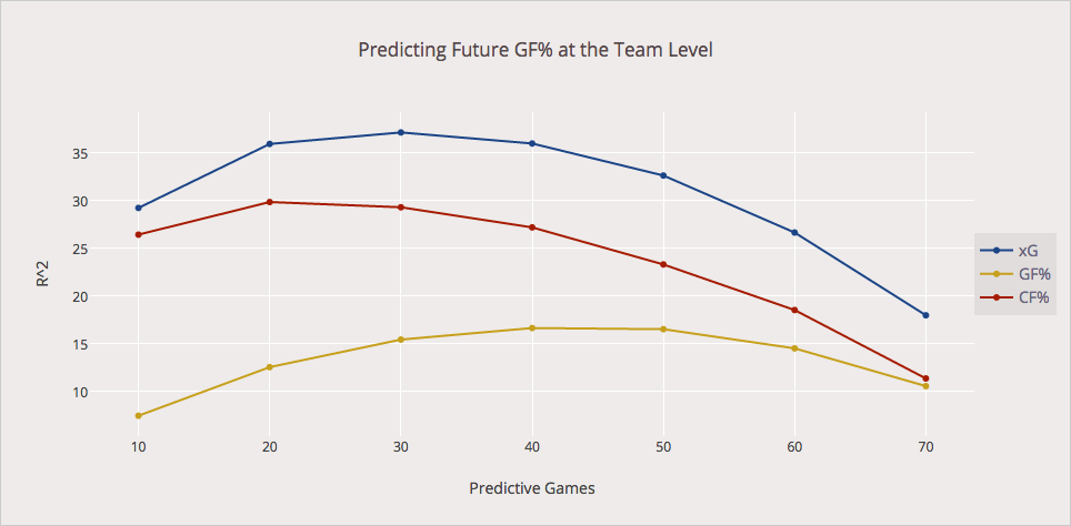
Figure 6

Excellent stuff. One minor quibble tho: I’m not sure adding in individual scoring talent (as your regressed shooting percentage does) allows you to still really call it “expected goals” – this makes it operate wholly differently than other versions of the Same concept . Not sure what you would call it.
How do the numbers change if you remove this component? In other words, how much of the improvement on team and individual levels comes solely from including actual shooting talent?
To the best of my recollection without the scoring talent aspect, xG is about on par with Corsi. I didn’t really explore that avenue at all. The impact of scoring talent / shot quality in general obviously seems to have more of an impact at the individual level. The original idea to include scoring talent came from this Eric T. article: http://www.sbnation.com/nhl/2013/12/12/5114366/nhl-stats-shot-quality-player-evaluation
This is probably the first time I’ve seen a #fancystat place a team above the 2007-08 Detroit Red Wings, which is intriguing.
Really interesting, and I think there’s good potential. One thing that comes to mind; in your in/out tests, we’re still seeing CF doing a strong job of predicting future CF, seemingly at a better relationship than xG to future xG. So, by getting a better predictor for GF, there’s still the practical hurdle of determining whether what’s being done to achieve a good xG is more repeatable relative to what’s being done to achieve a good CF. I’m probably just blowing the buried lede for Part II, but I’ll be interested to see the “sequel,” and how it addresses this.
Personally I think you should leave shooter talent out of the model. The issue with including it (although it will make your aggregate data look better and have a higher R2) is it actually obscures information. In your Brad Marchand vs Tanner Glass example, if they actually had the same expected goals for, of say 20, (pre shooter talent) then Marchand would end up with say 25 and Glass with 15. While this may end up lining up with the reality of what occurs, it doesn’t actually show that Glass was on the ice and generated chances that should have gone in 20 times.
What this means is, especially in the early days (i.e. 10 to 20 games into the season), you will essentially be predicting hugely high or hugely low for players who have good or bad luck. In the longer run this might even out (i.e. when you get to 30 or 40 games), but as we’ve seen with the Leafs it can take 50 or even 60 games before the wheels come off.
I think we need to think about the purpose of the analysis – is it to determine things we already can see (i.e. that the Leafs score a lot of goals in the first 30 games of the season) or is it to determine the ability of the team (or player) to continue doing that? i.e. to find things that are straying from our expectations and may revert back to them.
Again – good work. Just my 2 cents.
The GF and GA you are using in your chart is All situations — not 5 on 5 GF /Ga?
What am I missing?!
I believe that might be the regressed GF and GA, derived from 5v5 and using the K-R 21 formula, just not labeled as such. Not sure, though.
No if you look at the final table the results per team season include situations outside of 5v5. Not sure why. The K-R 21 formula should just be applied to determine individual shooter’s shooter multiplier (as described in the article). I’m not actually sure where they got the data for the final table.
For example, Pittsburgh 2011-2012 shows a GF of 222 vs GA 189 (54%). In 5v5 (my data) they were 185 and 157 (54.09%). Using War-On-Ice data I get 202-171 for 5v5 but ONLY if I could playoff games, 187-159 without it. If you add in 4v4 it’s another 10-6 (WOI Data) which is 212-177, again still not the same.
Similar discrepancies exist with other teams, but I’m not going to check them all.
I don’t think WOI includes OT which mine do. But yes it should read even-strength not 5v5 thank you for reminding me
Shot success is predicted by the # of open hole Med and High chance shots that are a defence pair allows a goalie to face and the Open hole med anfd High chance save % of each of the goalies.
Shooting a puck in glove/blocker then arm swing; Shot into pad; Shot into chest; Shot into helmet are zero chance shots. They are not going to go in.
Only Open hole shots requiring actual goalie movement can go in.
Shots have three quality’s
(LCS) low Chance outer circle to point. .9750 Save% @ even;
(MCS) Med chance slot .9250 Save% @ even;
(HCS) High chance shot .8330 save% at Even.
Team quality of defence leads to a variance of 5-8 HCS at even. 52% of even goals come from HCS @ even. You want D who reduce MED and HIGH chance shots @ even and PK since 84% of even golals come from that range.
You want the goalies that avg top 10 IN MED and HIGH chance shots @ even and PK. 2 have done that over last 2 years. Talbot and Schnieder.
Elite High chance Shot goalies last 2 years are Price; Halak; Varlamov And hiller added to the first 2.
Lange looked at predictive nature of shots and Quality.It is a waste.
Think shooting a gun at distance and targeting.
the location of shot and targeting quality of the shot.
Is about reaction time (keeping shot distance up) and not hitting the goalie (forcing lower trageting quality shots.)
Remeber Datsyuk’s shot targeting device. primeter from just above top of pad around the bar to other side just above pad level. A rebound in tight with alot of open area is just a open hole high quality shot.
A few questions/comments:
1. In the post you linked above, jlikens found that Corsi significantly out-predicts GF% throughout most of the season, but you chart above has GF% significantly out-predicting Corsi. Why?
2. Your chart has score-adjusted Corsi being far less predictive than Micah’s post linked above. Why?
3. We know that shot location is a large component of S%. But in your model you’re crediting players for their S% in addition to shot distance and angle. You seem to be crediting a player as much as three separate times for one thing. Even if that produces a result that looks nice, it strikes me as problematic methodology. You could extend that concern to some of the other things you’re looking at; for example, maybe a player has a high S% *because* they have a lot of tips and very few slapshots. I don’t know if this affects the results much, but it’s definitely something that sounds wrong.
1. I don’t know where you are seeing this. Figure’s 1 and 2 both have CF% greatly exceeding that of GF%.
2. I also don’t see this. Figure 1 shows SA-Corsi peaking in predicting future goals around the 20-30 game range (R^2 ~ 0.3), which is pretty much the exact same range on R^2 value Micah found.
3. The idea for the scoring talent portion comes from Eric Tuslky (http://www.sbnation.com/nhl/2013/12/12/5114366/nhl-stats-shot-quality-player-evaluation). Even after accounting for all of the contextual factors, many players still constantly exceed their projected scoring numbers due to their skill set (ex. fast release/especially accurate).
Looked at Figure 1 again. The legend is in a different order than the lines on the graph and somehow my mind crossed them when reading it. Obvious error on my part there.
On the scoring talent thing, though, I still think the method has problems. If you’re giving a player credit for shot location AND S%, you’re crediting (or penalising) players twice. Shot location is a major element of S%, so you need to figure out not just if a person shoot for a high %, but if they shoot for a higher % than expected given their locations (otherwise you’re counting the same data twice).
The Tulsky article you linked to doesn’t say anything about the particular elements you chose, it just says that there’s a small element of repeatability to shot delta. Note that among his conclusions is this sentence: “The shot quality factor just appears to add more noise than value over sample sizes of ~82 games, which is why these metrics have never really caught on.”
This bit, from Tulsky, especially as it relates to predictability at the team level, still seems accurate: “I like the simplicity of just using shot differential for my writing — it’s very nearly as precise and much simpler to explain.” The gap between xGF and CF at the team level seems pretty minor to me (enormously smaller than the gap between CF and GF).
I’m with draglikepull on this one. Unless there’s research that I’m missing, what’s not factored is how much affect the % of shots from the various danger zones has on the shooting % of the individual players.
So, for example, two players with a difference in sh% that can be entirely explained by ratio of HD/MD/LD shots, by this model appear to be credited with a natural shooting ability that actually doesn’t exist in reality, no?
Per one of the authors, the data in the table at the bottom of the article is wrong. I might suggest that it be removed or corrected.
I haven’t had a chance to read beyond Part 1 yet but great work from I’ve gone through so far.
The one thing that caught my attention though was the rationale that a shot attempted from a player’s strong side improves the likelihood of scoring.
Matt Cane presented some interesting research at the Pittsburgh Analytics Conference that seemed to conclude the opposite. Here is a link to the slides from his research:
Click to access 20141106_PGH_Analytics_Shot_Location.pdf
I believe we are referring the same thing. We just used different words. My On/Off Wing variable does in fact indicate something like the “Ovi shot” would have a higher likelihood of resulting in a goal.
Ah okay, yeah just a misinterpretation. Thanks!
I am a fan of the analysis however to better include average nhl fans ability to comprehend this artical I believe you need to expand the “glossary” of terms and abbreviations that are used in the formulas provide. I believe this will enhance the general fans understanding of the means of proofing of the stats found. Over all great artical but a little “heady”
Nice work, though I do find it strange how from 2012-2014 NJ was projected to be a great team but their final GF%s were way off. Can you think of any reason why that might be the case?