In part 1 of this series, I looked at how NHL skaters age using the delta method with Dawson Sprigings’ WAR model. As mentioned in my previous article, there is still one major problem with the delta method that needs to be addressed: survivorship bias. The “raw” charts presented in part 1 are quite informative, but they’re missing a correction for this bias. Before we can draw conclusions about what this new WAR metric tells us about NHL skater aging, we need to figure out how to correct for survivorship bias.

I don’t want to spend too much time defining what exactly survivorship bias is since it’s a well known type of selection bias, but the first paragraph of its wikipedia entry does a very good job summarizing the phenomenon (I know it’s Wikipedia but it’s good):

“Survivorship bias, or survival bias, is the logical error of concentrating on the people or things that ‘survived’ some process and inadvertently overlooking those that did not because of their lack of visibility… Survivorship bias can lead to overly optimistic beliefs because failures are ignored, such as when companies that no longer exist are excluded from analyses of financial performance. It can also lead to the false belief that the successes in a group have some special property, rather than just coincidence.”

With that in mind, we can start to imagine how this bias might influence our “raw” curves from part 1. It’s not clear to what degree this bias influenced the numbers, but we need to attempt to correct for this to find out. Mitchel Lichtman’s summary in part 2 of his piece here gives us a good idea of what this looks like in baseball:

“At every age, there is a class of players who play so badly in any one season that they don’t play at all (or very little, which I call “partial survivor bias”) the following year. (Obviously there are also players who don’t play poorly in Year I but also don’t play in Year II.) 

These players tend to be unlucky (and usually untalented of course, at least at that point in their careers) in Year I. Therefore the rest of the players who do play in Year I and the following year tend to have been lucky in Year I. This is survivor bias. Any player who “survives” to play the following year, especially if he racks up lots of plate appearances, whether they are good, bad, or indifferent players, true-talent-wise, will tend to have gotten lucky in Year I. In Year II, they will revert to their true talent level and will thus show a “false decline” from the one year to the next.”

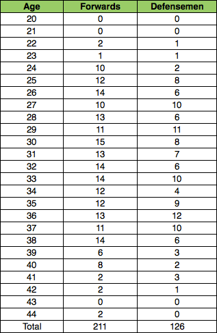
The thought experiment Lichtman lays out gives us a good place to start for, at the very least, identifying players who dropped out of the league – players who didn’t “survive”. Using this as the basis, I found all skaters who had at least two consecutive seasons of WAR data but did not qualify for the 2015-2016 season (to avoid considering players who may still be in the league). Here are the players who met this criteria at each age (I will call them “non-survivors”):

Here is the average change in Overall WAR for these players in their last Year I/Year II age couplet (the average change from their second-to-last season to their last season):

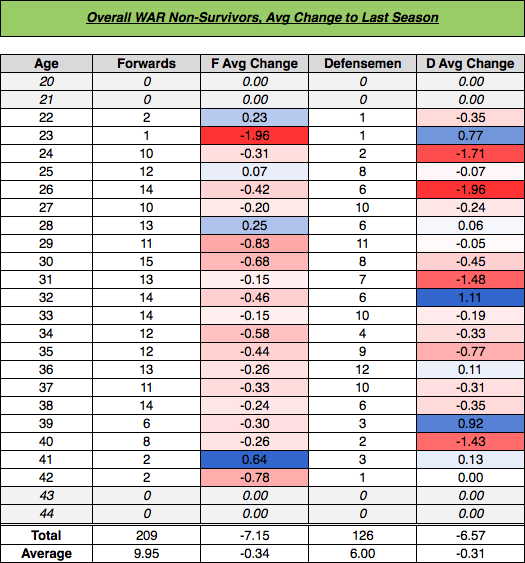
We can clearly see the average decline in performance these non-survivors experienced leading up to their exit from the league. Given what we know about survivorship bias, there were probably just as many equal “true-talent” players who didn’t experience the type of decline seen above (i.e. they got lucky) and survived to play another season.

So what do we do with all of this? How do we account for the non-survivors? What’s the best approach? These questions haven’t been definitively answered – the discussion regarding survivorship bias correction is still ongoing – but there have been several methods used in hockey over the last few years. I think it’s important to run through the work others have already done on this subject to help determine which method will work best for our purpose.

Background

Note: If the background of this subject doesn’t interest you, feel free to skip to the “Approach” section below.

As far as I can tell, Stephen Burtch kick-started the entire topic of survivorship bias in hockey with this article, where he argued that the Leafs should consider trading for Roberto Luongo. What followed was a series of fascinating back-and-forth articles discussing how aging should be approached in hockey. Eric Tulksy quickly (the same day) responded showing how Burtch had failed to correct for survivorship bias. Several days later, Petbugs13 offered his own take on the issue (“… comparing the performance of goalies as they age not to the league SV%, but to their own performance”). Burtch responded to all of this with an updated look at goalie aging that addressed some of the issues his original article had. Tom Tango posted this article to his blog, which generated a great debate in the comments (below you’ll see this is a trend). Funny after all of that, Luongo went on to put up stellar numbers in Florida, but I digress…

Most of this discussion dealt with goalies, and the methods proposed to correct for this bias were either limited or not applicable to skater WAR. A controversial study was published by Brander et al. (here) in the middle of this debate that utilized both the “elite performance method” based on Bill James’ work where only career arcs of elite players are used to determine peak age, and the “naive method”, which looks strictly at all players’ performance at any given age exclusively (don’t do this). Tulsky wrote a very interesting piece for the Washington Post questioning the methods and conclusions of the authors (they used +/-… not sure how an academic journal accepted a submission where +/- was so heavily relied upon) – so we’ll just ignore this approach. Tulsky expanded on a proposal he made in the Tango comment section above that looked at repeatability in hockey stats through simulations – this method is fascinating but difficult to adapt (Tulsky has explained that his methods at the time were intentionally vague due to editor restrictions, and he’s no longer in a position to help us anymore).

Tango (as we would expect) shared Tulsky’s article on his blog (here), which resulted in a certifiably gold comment section where Tango, Tulsky, Lichtman, and a couple others got into a long debate about seemingly everything we’ve already covered (including an imaginary fencing league devised by Tulsky to prove a point). As fascinating as that comment section is, it devolves fairly entertainingly into territory I’d deem unusable for our purpose, which might also mean it’s just way over my head (there might be something in there that I failed to identify, and for that I am sorry). All of this, however, led me back to Lichtman’s approach in part 2 of the Hardball Times article I quoted in the introduction, which I feel is the best approach we have for looking at and adjusting for survivorship bias using WAR (right now).

Approach

Lichtman utilized a method that projects “phantom” years for non-survivors, and he continues to be a proponent of an “additive” approach to correct for survivorship bias (along with Christopher D. Long and others). I don’t know if this is the “best” way to accomplish the correction we want, but I think it’s the best method we can utilize right now. It works like this: identify all players who dropped out of the league within the data, give them an appropriate “phantom” year after their last year, input those new seasons into our data, and re-calculate our initial aging curve. The question, then, becomes how do we “give them a phantom year”? Well, a projection system is probably appropriate for that. While I think there are a few options out there that might work, the best we can do in my opinion is adapt Tango’s Marcel projection system for hockey WAR.

Self-described as “the most basic forecasting system you can have, that uses as little intelligence as possible”, this projection system was created to offer a baseline that any other projection system should at bare minimum exceed – the “minimum level of competence that you should expect from any forecaster”. If you’re unfamiliar with it, please read Tango’s introduction. Lichtman actually used a method that is even cruder than Marcel, but baseball is spoiled and we don’t have a Marcel-type system for WAR projections that we can degrade. We will, however, attempt to set up our Marcel system to project seasons for these non-survivors in a way that accounts for their talent (they didn’t just stop playing due entirely to chance – they were most likely not very good to begin with).

In short, Marcel “uses 3 years of MLB data, with the most recent data weighted heavier. It regresses towards the mean. And it has an age factor.” There have already been a few adaptations of this projection system for hockey. Garik16 adapted Marcels for goalies (here and here), FooledbyGrittiness took this a step further and looked at L/M/H Sv% projections in this great article, Sprigings used Marcels to project team rankings a few years back (here), and DomG/MimicoHero adapted Marcels for skater stats (here). For our purpose, we’ll need to tailor this to WAR. Initially, I set up a system based on this article, and while I feel this method is much easier to apply to our data (and actually pretty close to what we want), it wasn’t close enough to Tango’s original projection system in my opinion (although I believe FooledByGrittiness showed this could be used if I was smarter). So I attempted to replicate Tango’s original Marcel method with A LOT of help from this Beyond the Box Score article. Please read these two articles if you’re unfamiliar.

The Process

Note 1: The following is math heavy. If that doesn’t interest you, feel free to skip the the “Charts” section below.

Note 2: I used the last season of all player data as n for both TOI and WAR weights, which is more conservative than what we’d probably want for normal projections. But seeing as we’re trying to project data for players who dropped out of the league, I feel this conservative approach is fair. I also realize there are some problems with translating Tango’s original system, but because our purpose is projecting phantom seasons, I think sticking to his original approach is appropriate for now.

The first thing we need to do is project TOI for all non-survivors. Tango’s original PA regression formula looks like this:

Projected PA = (n-1 * .5) + (n-2 * .1) + (200)

This needs to be adapted. I ran a multivariable linear regression for all players with at least 3 seasons of data to accomplish this. The last season for any player was treated as “n” (dependent) and the previous two seasons for each player were considered “n-1” and “n-2” respectively (independent). I did this for both forwards and defensemen, which resulted in the following weights for projected TOI:

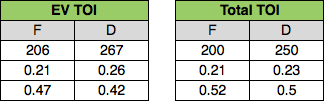
With these numbers, we can update Tango’s original formula for projected PA for our purpose of projecting TOI. For example, forward projected TOI in the Overall WAR projection calculation looks like this (the EV components use the EV TOI numbers):

Projected F TOI = (n-1TOI * .52) + (n-2TOI * .21) + (200)

We’ll set that aside for now. Next, I ran a similar regression for Overall WAR, EV Offense, EV Defense, and EV Overall to find weights for the weighted WAR portion of the projection (similar to DomG’s method in the article linked above). I used only players with four seasons of data to get three years worth of weights. I initially tried the standard 5/4/3 Marcel weights but found these were not ideal. Here are the weights I used to project WAR – forwards and defensemen were very similar so a regression of all skaters was used for simplicity:

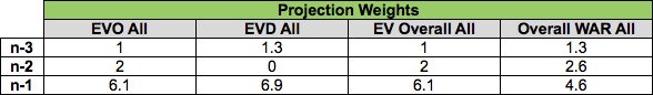
The regression component of Marcel adds in 1200 PA’s (600 PA given 2 weights) of league average PA for whatever component it’s projecting. Seeing as the weights I found differ from the standard 5/4/3 Marcel weights, I tried to keep the regression component intact by adjusting the amount of league average TOI we need to add (Marcel appears to regress everything by about ~15% – while this probably requires more work, I’m going to continue following Tango’s approach). This came out to a weight of 1.25-1.5 for both forwards and defensemen (I kept the amount regressed proportional based on the total of the weights). I’m treating Tango’s “600 PA” number as league average TOI for each position, which means we’ll take the average TOI per position and multiply it by the respective component weight to replace the 1200 PA’s (600 * 2) approach in Marcel for the regression component of the projection.

We end up with a formula that’s a little too long to lay out here, but it resembles the standard Marcel calculation (clearly shown here) with the above weights substituted and the number of league average WAR per any given player’s weighted TOI added in. This gives us a WAR per minute number (shown as HR/PA in the BTBS article), which we then multiply by the given player’s projected TOI from above to arrive at our pre-age-adjusted “phantom” projected season. For clarity, that looks like this (for forwards):

WAR per minute * ((n-1TOI * .52) + (n-2TOI * .21) + (200))

To tailor this for our non-survivors, I used 90% of the league average WAR rate per season (all player total component WAR per season / all player total component TOI per season) for the Marcel regression component. This was a mostly arbitrary decision based on Lichtman’s approach in adjusting the mean we’re regressing to downwards. This adjustment probably requires further investigation, but seems fair given our purpose.

Once we have this projected number, we apply an age adjustment. I used Tango’s original .006 increase to peak age and .003 decrease after peak age approach for this (step 5 here), and set the peak age at 25. This adjustment is fairly minor and could be altered. I’m ok with using this age correction method as it’s the standard method to adjust for age in Marcels, and we’re already using “last season” data to determine weights (which is more conservative) and 90% of the league average WAR rate to regress each player. I feel this is sufficient to project non-survivors.

With all that in place, I projected phantom seasons for all of the non-survivors using the above process, added these projected phantom seasons into the general population of all players that we looked at in part 1, and redrew the aging curve. I did this for Overall WAR, EV Offense WAR, EV Defense WAR and EV Overall WAR.

Charts:

Overall WAR:

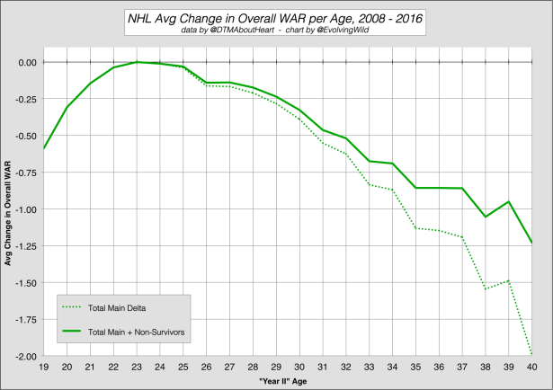
Overall WAR Total:

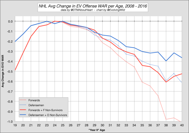
EV Offense:

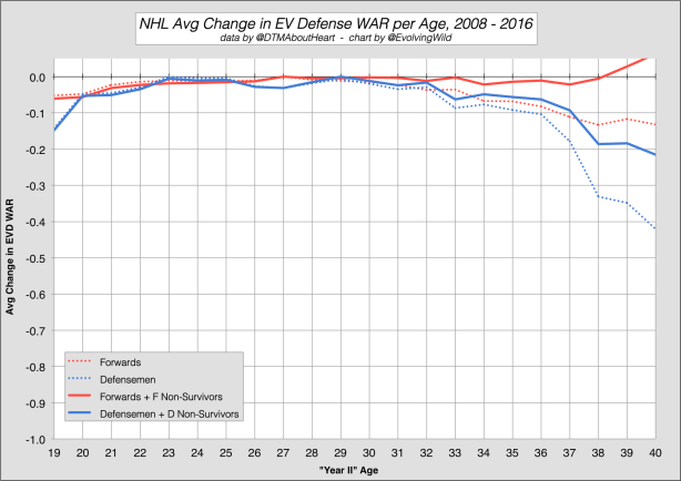
EV Defense:

EV Overall:

EV Overall Total:

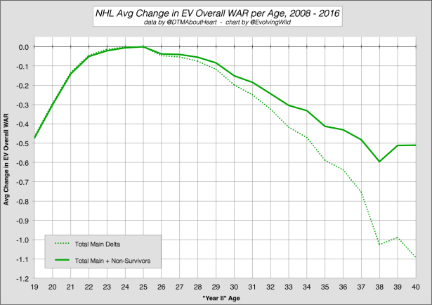
The first thing that sticks out is the lack of correction for players under 24 years old. Looking back at the total number of players identified as non-survivors, it’s clear we don’t have enough data to see an appreciable change for these ages. But it could also illustrate how teams rarely “give up” on young players (these players see reduced playing time or are demoted and do not qualify). If WAR measured “unqualified” players, I’d assume we would see the “peak year” shift to the right after the survivorship bias correction (like we see in other sports). If this were the case we could more accurately measure the decline of the lower-tier young players and correct for more non-survivors in this age range.

Another thing I’ve yet to discuss is the clear average decline from age 25 to 26 in all components – this creates something of a wall which prevents the “peak age” from shifting to the right. I think this is very interesting especially given the large number of players measured in this age couplet. At this point, I think the 25-26 drop is quite interesting and requires further examination – probably by comparing these aging curves to other metrics. But I will leave that for another article.

There are no charts for PP Offense, Taking Penalties, Drawing Penalties, or Faceoffs. After looking at the data and methods for correcting for survivorship bias, I determined that these components were not really suited for a correction using the above method. With powerplay offense, I feel that projecting “phantom years” for non-survivors doesn’t really make sense.The WAR component for PP Offense is rather strange in that it bottoms out at 0.00 WAR (essentially, a player will at worst add no value on the powerplay). Players in the non-survivor group averaged 95 minutes of PP TOI in their careers, but only 444 of the 1259 player seasons were above 0. Honestly, I don’t know if powerplay offense WAR suffers from survivorship bias to a significant degree, or at least with the data we are measuring. Tulsky has argued it does (here), but there are constraints to PPO WAR that would require a significantly different approach, and I am not going to do that here.

Lastly, the average change per age in the taking and drawing penalties components showed a lot of variance. Adding in projected seasons for non-survivors in these components only exacerbated this. While I think it’s important to look at how players age in these components, I found creating “phantom years” problematic. And honestly, there is so much randomness (and venue issues and the subjective nature of penalties in general, etc.) in taking and drawing penalties that I’m not sure survivor bias effects these components to a significant degree.

I guess I didn’t really cover the faceoff component, but (as you might remember) the change was so small year-over-year (and its total value in comparison to the other components is so small). For now, I’m going to deem a correction unnecessary.

Final Thoughts:

The method we used to correct for survivorship bias seems to have done a reasonable job given the limitations of the data available. However, the delta method will always have flaws – even after addressing this bias. Lichtman has pointed out that an aging curve constructed using the delta method represents a “hybrid” player, and this by itself is an issue. Additionally, our data starts in 2008, so we are unable to include the full career of any player who has played more than 8 years in the NHL (we cannot include Jagr’s entire career, for instance). I think it’s important to note that this is an average change and not the expected change for every single player. Additionally, with any analysis of player aging there will always be players who “defy” the curve, so to speak, and that should be taken into account when looking at any given player. Regardless, I do think this approach could be applied to projection models for WAR as a potential age adjustment (like we used in the Marcel projection above). While it’s not ideal (it seems no age adjustment ever is), I think it’s more accurate than the age adjustment Marcel utilizes.

Given what we know about NHL skater aging based on various methods and approaches (which I covered in more detail in part 1), I find it very interesting that this WAR model, for the most part, lines up with the generally held belief that skaters peak around 24-25 years old and decline gradually after that (there does seem to be some indication here that the decline of players over 30 might not be as steep as is often assumed). While some of the individual components do not show this, the EV Overall WAR and Overall WAR numbers do – I might argue they strengthen this notion. As we get more data, these curves may change, but for right now EV Overall WAR and Overall WAR seem to support what we already know. From an aging perspective, this metric makes sense. In my opinion, that alone lends credence to its validity.

_________________________________________

I’d like to thank:

• Mitchel Licthman for providing additional information that helped me better understand survivorship bias (and for the fantastic pieces he wrote about aging curves)
• Dawson Sprigings for providing additional insight into specific aspects of his WAR model
• DomG, Garik16, and Tom Tango for helping me adapt the Marcel projection system for hockey WAR   
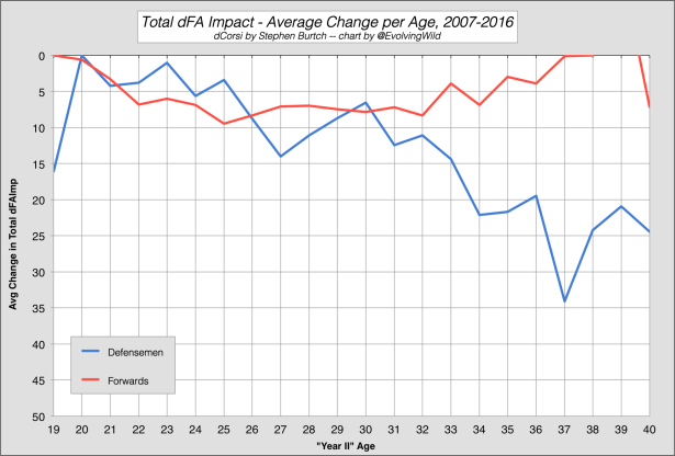
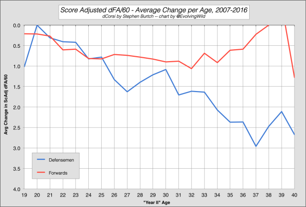
• Stephen Burtch for providing me with the historical dCorsi data that you will see below

…

Addendum – (EV Defense): 

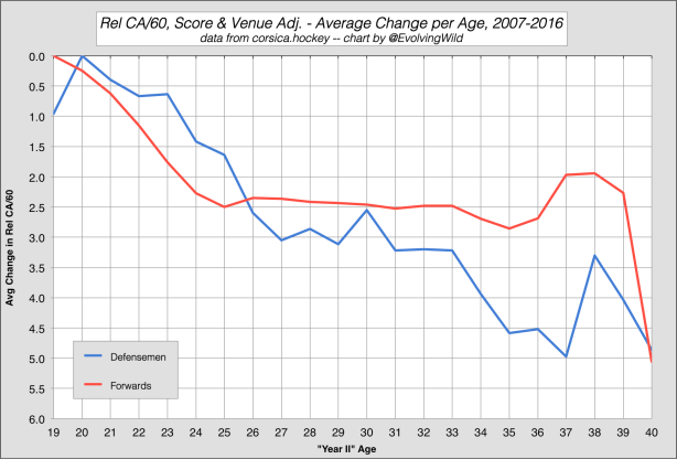
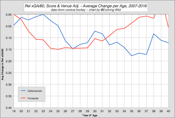
After part 1, there was some discussion about the lack of change year-over-year in the EV Defense component of WAR. Because of this (and the known difficultly in accounting for individual defensive contributions), I thought I’d make some aging curves using other metrics that are commonly utilized to measure defense. Below, I constructed aging curves for Relative Corsi Against per 60, Relative xG Against per 60, and two metrics from Stephen Burtch’s dCorsi (Total Fenwick Against Impact and Score Adjusted Fenwick Against per 60) – all of these are 5v5 metrics. These are raw age curves – I did not attempt to correct for survivorship bias here. Additionally, I used only “qualified” player data (top 390 forwards and 210 defensemen – 5v5 TOI) to keep the pool in line with WAR.

Relative Corsi Against per 60:

Relative xG Against per 60 (corsica):

Total dFA Impact:

Score Adjusted dFA/60:

And, for comparison, here is the EV Defense WAR graph from above with an adjusted scale:

At best, these appear to support the fact that our ability to measure individual defensive contribution still has room for improvement. They appear to show that defense may actually be, on average, more of an inherent talent than a skill that one can improve on as they age. The forwards do appear to show something of a plateau, but the defensemen are all over the place. But honestly, I’m not really sure (and don’t want to make any concrete claims here). In my opinion these charts don’t really prove much other than to show EV Defense WAR is essentially no different than the metrics commonly used to measure a skater’s defensive ability.