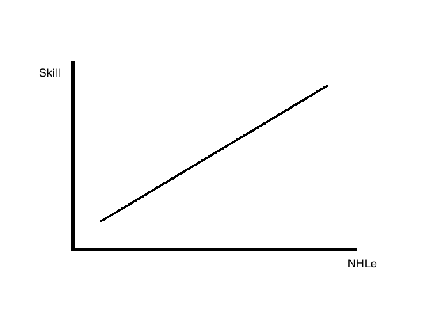
The graph above represents how some may look at and use hockey statistics; the better a player performs in a statistic equates to more skill. This practice can be found in league equivalencies -now more commonly known as NHL equivalencies (or NHLe)- originally contrived here by Gabriel Desjardins.

In truth, almost all of us can be guilty of this at one point or another, like when using evidence like “Player A has a better Corsi%; therefore, he is pushes the play better”. Most reasonably understand that this is not how it works, but it is not discussed often enough. These tools are used to show average expected outcomes. The output is not the only possible outcome. 

What does this have to do with analytics and drafting?

Open the image in a new tab for expanded image. Apologies to those colour blind and cannot find the blue and red dots.

The graph above displays the basic theory behind NHLe. The greater a player’s point production relative to their league strength, the more likely a player is a better point producer at the next level.

The key word is likely.

The dots on the graph represent all the actual outcomes. They are often very close or on the line, but not always. The line represents what you expect for the average player with that NHLe. Sometimes there are dramatic shifts. There are two dots on the graph above coloured red and blue as an example of a player having a lower NHLe, but ultimately leading to more production in the future than another player with a higher NHLe.

Like any quality regression curve, the density of dots is greatest at the line and disperses as you move further away. This indicates the most probable outcomes are at the line, and become less probable as you move out, like a probability density curve.

Where do we go from here?

There are many reasons why we see these differences. The NHLe model lacks contextual nuances like deployment (ice time, line mates, line matching, power play time, zone deployment, etc.), personal and on-ice shooting percentage variance, age, size, era, and other factors.

Not long ago, Rhys Jessop and Josh Weissbock worked on improving juniour scoring production measurements by adding age and era adjustments to help account for some of these missing items.

However, modelling does not have to limit itself to quantitative data. Qualitative information -like traditional scouting- still has a lot of value.

This graph made by Matt Pfeffer shows the value (in GVT) of all skaters at each draft selection. While imperfect like all things, traditional qualitative amateur scouting has a history of doing pretty well. There is value there and to dismiss it would be perilous.

The right way would be integrating the two methods, which would look a bit like this:

Open image in new tab for expanded image. Apologies to those who are colour blind and cannot find the blue and red dots.

We have a theoretical regression curve like before where a player’s statistical performance is estimating their skill level and future potential. The statistical model would simply expect the most likely outcome at the line. However, here we have added some qualitative information.

Whatever the reason -maybe character, skating technique, hockey IQ, play style, pedigree, whatever- scouts predict that one player is likely better than what the quantitative data indicates, while the other is likely worse. The thick region is where the scouts indicated was the most likely outcome.

The issue with adding qualitative data into a quantitative model comes with testing. How do you know you are doing well in evaluating talent?

You test the new model’s performance against the quantitive only model.

Jessop and Weissbock performed something like this when they compared a few statistical models against all 30 NHL team’s drafting performance.

Where are we today?

Here is a look at AHL points per game versus next season’s NHL points per game for all players who played at least 40 games in each from 1940 to 2011. All data is from Rob Vollman and can be found here.

We see that even without any of the added information of context, era differences, shooting percentage regression, or qualitative scouting, the model already explains just over 30% of the outcomes -as shown by the R-squared- and the relationship is significantly strong -as shown by the Correlation Coefficient-.

With the addition of these missing elements, a team can not only improve their amateur scouting, but also effectively test their scouting department’s performance.

Random note: There is a slight downward slope at the AHL maximum for the Studentized Residual Plot (not shown), hinting that the model loses linearity at the highest scoring AHL players. There are diminishing returns. In layman terms, as you move into the highest scoring AHL players, any additional improvement in AHL scoring becomes less of an impact in their NHL scoring.