Every once-in-a-while I will rant on the concepts and ideas behind what numbers suggest in a series called Behind the Numbers, as a tip of the hat to the website that brought me into hockey analytics: Behind the Net.

Almost weekly, you will see a “quant” or “math” type complain about some of the binning going on (usually with Quality of Competition or scoring chances).

But the reason may not seem intuitive, so I’ll use scoring chances as an example and explain the issues with binning continuous data.

I will start off by saying that binning is not altogether bad, just inferior to actually modelling the continuous variable.

So, what is binning?

Binning is simply splitting some population data into groups by setting some semi-arbitrary lines. Scoring chances and non-scoring chances splits shots into two bins. We know that the average shot taken at the blue line is less likely to score than a shot 5 feet in front of the net, so we put them into two different buckets to distinguish them. But this bucketing gets harder and more arbitrary when you look at shots in the middle of two extremes.

If you were to ask 30 coaches the definition of a scoring chance, you will get 20 or more different answers. Commonly in the blogging community we see scoring chances classified as shots within the “home-plate” area like the above title image.

Unfortunately, individuals often make the wrong choice and toss out the less optimal area. Sure the average scoring chance matters more than the average non-scoring chance, but shots outside still have a significant impact on winning games.

Using Super Shot Search, we see that shots in the home-plate area score about 14 percent of the time and account for about 78 percent of the goals despite only accounting for about 46 percent of the shots. However, the missing around 22 percent of goals still matter. In addition, some scoring chances arise from rebounds or tips from non-scoring chance shots.

Ignoring some shots can give you an inaccurate picture of how a team is performing.

In the next image, I have provided an extreme example of how looking simply at scoring chances could potentially obscure what is truly going on with the distribution of five shots:

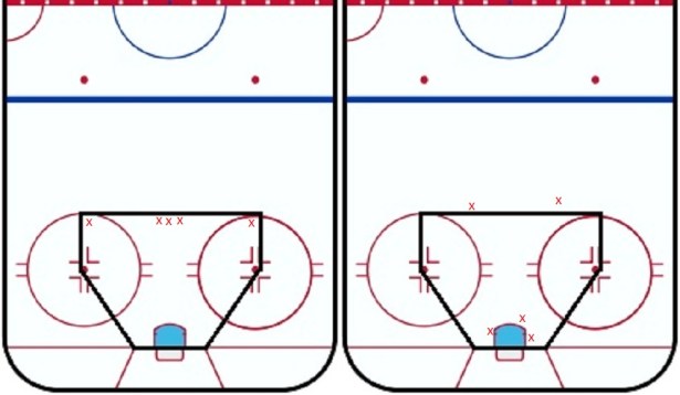
Most observers would rather their team got the five shots on the right than the five on the left, given all other factors being equal. But if you look only at scoring chances, you’ll think the left team’s five scoring chances were better than the right team’s three. This is the danger with binning: it counts nearby shots on either side of the line as very different, and shots on opposite ends of the home plate area as exactly the same.

In the long run huge discrepancies likely wash out; however, the data will be non-optimal. Also, coaches and teams often enjoy scoring chance data over single games.

Typically the solution for teams is to increase the number of bins. Commonly we see teams evaluating player given with “prime” or “non-prime” scoring chances. Another option is “graded” scoring chances where a player can generate an “A” grade chance or “B” grade chance.

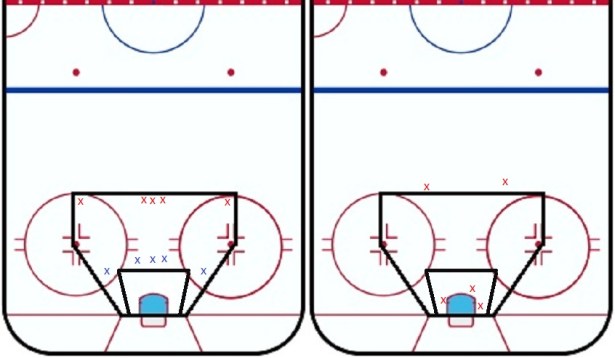
Increasing the binning by creating a “prime level” scoring chance area would help with our last example, but still you can see potential issues:

This is where statistical modelling comes in. A statistical model, like expected goals, simply creates nearly a nearly infinite number of bins. Every possible location becomes its own bin.

Modelling also allows one to weight each bin appropriately by their ability to predict goals. No longer are any shots arbitrarily worthless, instead they are worth their ability to produce goals. A shot from the blue line may only go once in a hundred times, but you will still be more accurate with a statistical model that counts it as 0.01 of a goal than a bin that counts it as 0.

This also makes accuracy in shot location less important, although precision still matters just as much. If specific arenas tend to have a bias, you can adjust for that. If all scorers tend to push shots in a particular direction (due to some inherent human bias), the model’s weighting of the false location will be the same as the weighting of the true location if all shots were not pushed in that direction. Precision issues would still require a certain sample to wash out small sample variance. (Click here for the difference between accuracy and precision)

Overall, there is no reason to bin when you can use a sophisticated model. While a model may not be able to account for all variables that causes one shot to be worth more than another, it will still vastly outperform someone subjectively creating their own value to each shot.

Another area where this occurs is Quality of Competition binning. Individuals may arbitrarily split a player’s performance against different groups of opponents.

The same issues come along:

• Looking how a player performs just against the best is missing minutes that still matter
• Binning the top ‘X’ amount of players assumes that all players in that group are equal, and the next one following them is totally different
• A sophisticated model removes subjective bias in evaluating which players are the best

I do acknowledge the previous issues with QoC and QoT variables were using only the mean value for a distribution, but looking just at one portion of the distribution does not necessarily improve upon that. Regression models will still be superior to either alternative.

I will leave you with this final point: this whole article revolved around the issues with binning continuous data. These same issues do not exist with binning non-continuous, or discrete, data. For example, when we split a player’s performance 5v5 versus 5v4 situations, the line is not arbitrary.

For a deeper statistical and theoretical reasoning why binning continuous data can be problematic in general, click here.