
If you’ve ever read a little math, you likely know the dangers of binning continuous data when testing relationships between two variables. It is one of the easiest and most common mistakes that an amateur statistician might make, largely because, intuitively, it seems like it should make sense.
But it doesn’t, and here’s why.
Ok, sometimes it does. You can bin data when there are logical, discrete “breaks” in the data based on a physical characteristic. For example, if you wanted to analyze the likelihood a given shot will result in a goal, it’s perfectly fine to create bins for shot type to distinguish slap shots from wrist shots, one-timers, deflections, rebounds, etc. There are discrete, physical distinctions between these shot types that create logical bounds to the bins. Similarly, it makes sense to bin across things like team strength (5v5, PP, PK, etc.) and even score, because there are distinct, discrete breaks in the data (tied, up 1, down 2, etc.).
But what doesn’t make sense, and is statistically problematic, is to arbitrarily break continuous data into bins just to make it easier to analyze. So going back to the shot example, binning shots by location on the ice can seriously undermine the validity of your results. The fewer the bins, the greater the problem. Similarly, binning players by ice-time can also undermine the validity of the results, depending on the the conclusions being drawn.
To illustrate the problems with binning, let’s take a look at something I have previously done some research into: how team performance varies with game pace. I’m not going to get into the topic itself, but for some basic background “pace” is defined as the sum total of all shot attempts (for + against), per 60 minutes of game play and “performance” is measured by the goal differential (for – against) per 60 minutes of game play.
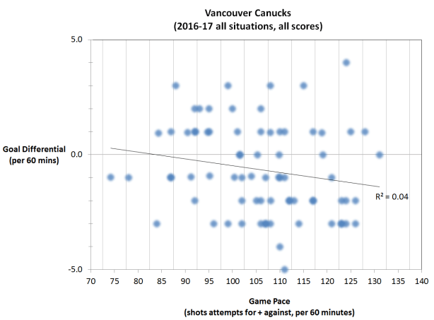
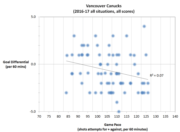
If we look at the Vancouver Canucks’ season through March 28, 2017 it looks like this:

Each data point represents one game, and the game pace is plotted as a continuous variable along the x-axis. The linear regression trend line indicates that there is a slight negative relationship between pace and performance for the Canucks, which intuitively makes sense. They are not a very good team, and slowing the game down is their best chance of getting positive results. But the relationship is not very strong, as you can see from the spread of the data points and as indicated by the low R^2 value.
The temptation though, is to bin games together. There isn’t much difference between a 110 and 112 pace, so why not put those together to give us a bigger sample of those types of games? They’re pretty much the same, right? So why not break the data into 5 shot attempt wide bins. That seems like a good size to still provide some distinction between bins but also give us bigger samples in each bin:
So we wind up with bins centred on every 5 shot attempts, and now we can compare a game with a pace of roughly 85 shot attempts per 60 to one with 125 shots attempts per 60. How? Well, we add up all the goals for and against and calculate an average goal differential for each bin:
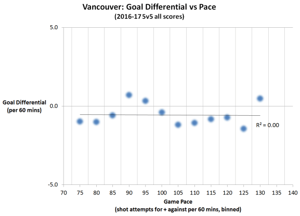
You can see that by doing this, you lose all sense of the variance in the original, continuous data set. And in this particular case, averaging the bins eliminates the correlation between game pace and goal differential altogether. Often it does the exact opposite, which is to make the correlation much stronger than when using continuous data.
In fact, we can get there even with this particular data set. Another poor data management practice that is often used hand-in-hand with binning, is to trim the tails of the continuous data.
In this particular example, you can see in the original chart that there were many more games in the 90 to 120 pace bins than in those below 90 and above 120. So what if we tried to represent that by sizing the data points for each bin proportionally to the total TOI for all the games in the bin:
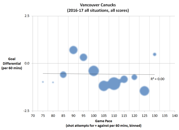
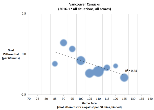
Ok, now it is abundantly clear that there were very few games that fell in the 70, 75, and 130 pace bins, so why should they have just as much weight as all the other bins that had so many more games in them? This is where the temptation to think those bins clearly have too few samples and should just be discounted comes in. And once that happens, all is lost:
All this to say, reading a little math is a dangerous thing. But it’s still better than reading none at all.
ADDENDUM:
A suggestion has been made, that the problem isn’t with the binning, but rather with the cropping of data. Here is what the continuous data looks like if you crop the same data out:
So maybe it’s not the cropping after all. There’s really no purpose in cropping the extremes at each end when working with continuous data, but doing so, in this case, only slightly increases the strength of the relationship. Binning, on the other hand, hides any sign of variance in the results and, in this case, also erases the small relationship that does exist. If anything, it’s the two together, that create the problem in this example, but binning can definitely do it all on it’s own.
Now, don’t get me wrong. Removing outliers is still really, really bad practice and I’m glad to see that people are finally realizing that it too can produce exaggerated correlations.
You can read more from petbugs here, or follow on Twitter: Follow @petbugs13
