Note: In this piece, I will use the phrases “scoring rate” and “5on5 Primary Points per Hour” interchangeably.

Introduction

Nico Hischier and Nikita Kucherov are both exceptional talents but suppose, for whatever reason, we want to identify the superior scorer of the two forwards. A good start would involve examining their 5on5 scoring rates in recent seasons…

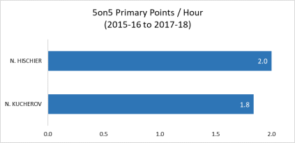
Evidently, Hischier has managed the higher scoring rate but that doesn’t convey much information without any notion of uncertainty – a significant issue considering that the chunks of evidence are of unequal sizes. It turns out that Kucherov has a sample that is about three times larger (3359 minutes vs. 1077 minutes) and so it is reasonable to expect that his observed scoring rate is likely more indicative of his true scoring talent. However, the degree to which we should feel more comfortable with the data being in Nikita’s favor and how that factors into our comparison of the two players is unclear.

The relationship between evidence accumulation and uncertainty is important to understand when conducting analysis in any sport. David Robinson (2015) encounters a similar dilemma but instead with regards to batting averages in baseball. He presented an interesting solution which involved a Bayesian approach and more specifically, empirical Bayes estimation. This framework is built upon the prior belief that an MLB batter likely possesses near-league-average batting talent and that the odds of him belonging to one of the extreme ends of the talent spectrum are less likely in comparison. As evidence is collected in the form of at-bats, the batter’s talent estimate can then stray from the prior belief if that initial assumption stands in contrast with the evidence.  The more data available for a specific batter, the less weight placed on the prior belief (the prior in this case being that a batter possesses league-average batting talent). Therefore, when data is plentiful, the evidence dominates. The final updated beliefs are summarized by a posterior distribution which can be used to both estimate a player’s true talent level and provide a sense of the level of uncertainty implicit in such an estimate. In the following sections we will walk through the steps involved in applying the same empirical Bayes method employed by Robinson to devise a solution to our Hischier vs. Kucherov problem.

The Likelihood Function – Compiling the Evidence

The framework begins with defining a function that encapsulates the evidence provided by a skater’s recorded scoring history. When utilizing the Bayesian method, the mechanism which accomplishes this task is called the likelihood function. In this case, the likelihood function will divulge the relative likelihood of a skater possessing any specified underlying true scoring rate given the available evidence.

Building the likelihood function requires an understanding of the process through which primary points are produced. More specifically, this entails determining the underlying probability distribution that generates the data. In certain cases, the number of events observed in a given period of time follow a Poisson process. This type of process describes events that meet the following criteria…

• Events are memoryless: The probability of an event does not depend on the occurrence of a previous event (Ryder, 2004, p. 3)
• Events are rare: The number of opportunities to produce an event far exceed the number of events that actually occur (Ryder 2004, p. 4)
• Events are random: Events occur in time with no apparent pattern (Ryder, 2004, p. 4)

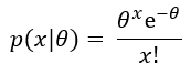
Goal scoring in hockey certainly seems to satisfy these properties and so it should not be surprising to learn that goals are approximately Poisson distributed (Ryder, 2004). We are concerned with primary points – the goals scored in which a skater managed to be the scorer or primary passer. For now, let’s assume that primary points are also Poisson. The implication is that if we let θ represent a skater’s true underlying scoring rate per hour, then the probability of that skater managing to tally x primary points in one hour of 5on5 ice time is defined by the Poisson distribution…

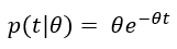
The Poisson process can be framed differently. Suppose scoring is Poisson and a skater’s true scoring rate, θ, is known. The probability density or relative likelihood of t hours elapsing between any given two primary points is instead modeled by the exponential distribution…

Whether or not the time between scoring in the NHL is actually generated by an exponential distribution can be tested with the Shapiro-Wilk Test for exponentiality (Shapiro & Wilk, 1972). The null hypothesis is that the data is exponential, and the significance level of the test is 5%. This means that for a skater’s sum of points to be rejected as being generated by an exponential distribution, his points must follow a pattern in time that deviate from exponential expectations to a degree that would occur less than 5% of the time if the data were in fact exponential. Controls are created by generating artificial time distributions from both a true exponential distribution and a chi-squared distribution (1-degree of freedom) for each skater. If our data is exponential, it should mimic test results of the actual exponential distribution and compare favorably to the chi-squared distribution.

Applying the Shapiro-Wilk Test ten times to all skaters who have spent a single season as an NHL regular and have recorded 10 or more primary points over the past 3 seasons produces the following result…

Given that the significance level of the test was 5%, the 5% rejection rate for the exponential distribution is as expected. The skater scoring data has a slightly higher rejection rate of 5.7%, meaning that it is not perfectly exponential, but close. The chi-squared distribution was effectively snuffed out by the test as it was rejected in over half of the randomly generated samples. Separating forwards and defensemen produced similar results. Overall, it is concluded that the time between 5on5 primary points can be approximated well enough by the exponential distribution but further testing is warranted.

Moving forward, the likelihood function for skater scoring rates will be constructed assuming that an exponential distribution generated the data. Every time a skater manages to gain a primary point, the time it took for him to do so is noted. The excess time left between the skater’s most recent primary point and the moment he last got off the ice is simply added to the time it took to score the skater’s first primary point (this is perfectly acceptable thanks to the memoryless property of the exponential distribution). Each one of those lengths of time is a piece of information that says something about the skater’s scoring talent. A player’s collection of primary points and the time required for their production are treated as independent, identically distributed exponential random variables. They are combined into a likelihood function which, as stated previously, unveils the likelihood of a certain underlying scoring rate (θ) given the evidence/data…

Using some basic calculus, we can find the scoring rate with the greatest likelihood conditioned on the available evidence for any given player. For this likelihood function, it turns out that it will always be a player’s observed scoring rate over the entire sample. Due to sample size issues in particular, it is clear that such an estimate would be unsuitable in many cases. The problem is that the likelihood function is initially completely agnostic to any potential scoring rate from 0 to infinity. Of course, there is plenty of historical data that can help identify which scoring rates are feasible over a 3-year period in the NHL. Incorporating that prior information can improve estimates and increase precision. The next section will tackle the process of defining prior beliefs with the aforementioned historical data.

The Prior Distribution – Defining Prior Beliefs

The choice of a prior distribution is completely subjective. This subjectivity goes as far as defining priors rooted in psychological probability, as long as these probabilities are coherent. Empirical Bayes is an approximation to a proper Bayesian hierarchical model and it involves estimating the prior distribution from the data itself. Using the data/evidence to define prior beliefs is certainly contradictory, but the method works as long as each individual data point used to estimate the prior is one of many in a large collection of data points. For example, fitting a prior distribution to the entire population of NHL skaters minimizes the influence of any single skater to the point where the prior can be thought of as roughly independent from each individual in the data set.

The aim is to fit a prior distribution to the scoring rates of forwards and defensemen (60+ games played) over a 3-year span. The data set will be composed of three 3-year blocks encompassing the following seasons… 2009-10 to 2011-12, 2012-13 to 2014-15 and 2015-16 to 2017-18. Scoring rates in each time interval are slightly adjusted so that the means are consistent with the latest of the three intervals. Also, skaters will share the same prior with individuals who play the same position. This will amount to initially assuming that every NHL skater is of league-average ability, with a distinct notion of uncertainty associated with that assumption depending on the skater’s position (forward or defense).

Let’s plot the data…

It is common to use a gamma distribution, a generalisation of the exponential distribution, in cases where the likelihood is exponential/Poisson. The gamma is a convenient choice as it supports only positive values, is very flexible and makes sampling from the posterior distribution (our updated beliefs) extremely simple. The gamma distribution is an appropriate choice for defenders in this case. Forwards, on the other hand, are clearly not gamma-distributed. The forward data instead favors a different generalisation of the exponential – the Weibull distribution. Both distributions are fit using a maximum-likelihood approach with the MASS package in R. The same distributions are shown below but this time they are overlaid with their fitted priors…

A good fit in both cases but it should be noted that typically the choice of prior distribution is further supported by a theoretical understanding of the process underlying the data. Unfortunately, there is very little theory associated with the expected distribution of scoring talent in the NHL that would tempt one to prefer a Weibull rather than a gamma, for example. The approach used in this piece relies solely on the range of supported values and a reasonable fit with the data. This process can lead to over-fitting. However, since the sample of historical data is large, over-fitting the data is less of a concern.

The Posterior Distribution – Consolidating the Evidence and the Prior

The final distribution, the posterior, represents an updated belief about a skater’s true scoring rate and is proportional to the product of the likelihood function multiplied by the prior distribution.

The proportionality preserves the relative likelihood differences between scoring rates. This allows us to combine all terms which do not concern the scoring rate into a constant and effectively ignore them. The final forward posterior density with respect to any given scoring rate (θ) is defined as follows…

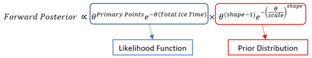
*The shape and scale parameters of the prior distribution were earlier determined when fitting the Weibull prior to the historical data set

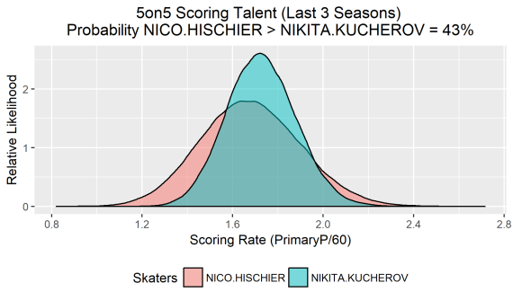
The posterior provides all the information necessary to deal with the Hischier vs. Kucherov scenario mentioned earlier. For each skater, it associates a relative likelihood with any given scoring rate. For example, a scoring rate with a relative likelihood of 2 is twice as likely as a different rate with a relative likelihood of 1. Of course, there is only one true scoring rate for each player and so the posteriors allow us to sample a single rate for both forwards. By repeatedly sampling rates and keeping track of how many times Hischier rates higher than Kucherov, one can estimate the probability that the former is the superior scorer. Taking 100,000 samples from each posterior (using rejection sampling), it is found that Hischier is the preferred scorer in about 43,000 cases. This implies that that there is only a 43% probability that Nico is the better scorer, despite the fact that he possesses the higher observed scoring rate (2.0 PrimaryP/60 vs. 1.8 PrimaryP/60). We can plot those 100,000 samples and form approximations of each posterior distribution…

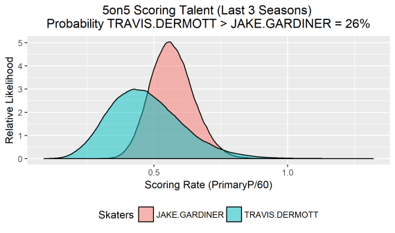
Knowing the probability that one skater is the more efficient even strength scorer is significantly more enlightening than simply eye-balling their raw scoring rates and respective sample sizes. We can generate the same plot for any two skaters, as long as they play the same position. Here is Travis Dermott vs. Jake Gardiner…

You can find the code used to compute the posteriors and generate the comparison plots HERE. Instructions on how to use the provided functions to compare skaters are included.

Sources

Robinson, D. (2015). Understanding empirical Bayes estimation (using baseball statistics). Retrieved from http://varianceexplained.org/r/empirical_bayes_baseball/

Ryder, A. (2004). Poisson Toolbox: a review of the application of the Poisson Distribution in hockey. Retrieved from http://hockeyanalytics.com/Research_files/Poisson_Toolbox.pdf

Shapiro, S.S. and Wilk, M.B. (1972). An analysis of variance test for the exponential distribution (complete samples). — Technometrics, vol. 14, pp. 355-370.

More applications of empirical Bayes in sports

Alam, M. (2016.). How good is Columbus? A Bayesian approach. https://hockey-graphs.com/2016/12/27/how-good-is-columbus-a-bayesian-approach/

Yurko, R. (2018). Bayesian Baby Steps: Intro with JuJu. http://www.stat.cmu.edu/~ryurko/post/bayesian-baby-steps-intro/